SPSS Statistics Assessment: Quantitative Methods in Social Research
VerifiedAdded on 2020/07/22
|19
|3784
|116
Homework Assignment
AI Summary
This SPSS statistics assessment delves into quantitative methods in social research, utilizing the SPSS software for data analysis. The assignment covers various statistical concepts, including levels of measurement (nominal, ordinal, interval, and ratio), central tendency, dispersion, and frequency distributions. It explores the impact of variable measurement levels on statistical analysis, and presents descriptive statistics such as mean, mode, standard deviation, and variance. The assessment includes analysis of survey data related to topics such as tax loopholes, awareness of environmental organizations, working hours, retirement age, and educational attainment. Statistical tests like ANOVA are employed to assess relationships between variables, such as the impact of sex on transgender beliefs and the relationship between race and car ownership. Additionally, the assignment covers sampling distributions, statistical inference, confidence intervals, regression, correlation, and proportionate reduction in error (PRE), providing a comprehensive overview of statistical analysis techniques and their application in social research.
SPSS Statistics Assessment Quantitative
Methods in Social Research
Page 1 of 19
Methods in Social Research
Page 1 of 19
Paraphrase This Document
Need a fresh take? Get an instant paraphrase of this document with our AI Paraphraser
Table of Contents
1(A). Different levels and their properties...................................................................................1
1(B). Listing level of different variables......................................................................................1
1. (C). Impact of variables level of measurement on statistical analysis.....................................1
2(A) Two dispersion and central tendency measurement............................................................1
2(B). % of respondents heard of Greenpeace..............................................................................2
3.(A) Greatest number of hours on normal working....................................................................3
3(B). Recoding to display proportion of percentage working for different time duration...........3
3.(C). % of respondents strongly agreeing across people working more than 60 hours..............4
4 (A). Confidence interval for the men age of retiring................................................................6
4(B). Mean age of people in completion of continuous full time education...............................7
5.(A) Sampling distribution.........................................................................................................8
5. (B). Role of sampling in statistical inference...........................................................................8
6.(A). Impact of sex over transgender people’s belief.................................................................8
6.(B). Statistical significance between cars and vans owned by people differ by race................9
6.(C) Association between respondents and adults watching pornography...............................10
6.(D). Mean % of hip replacement patients across men and women.........................................11
7. (A). Regression......................................................................................................................12
7.(B). Correlation.......................................................................................................................13
7.(C). Scatter plot.......................................................................................................................14
7. (D). Proportionate reduction in error (PRE)..........................................................................15
REFERENCES..............................................................................................................................15
Page 2 of 19
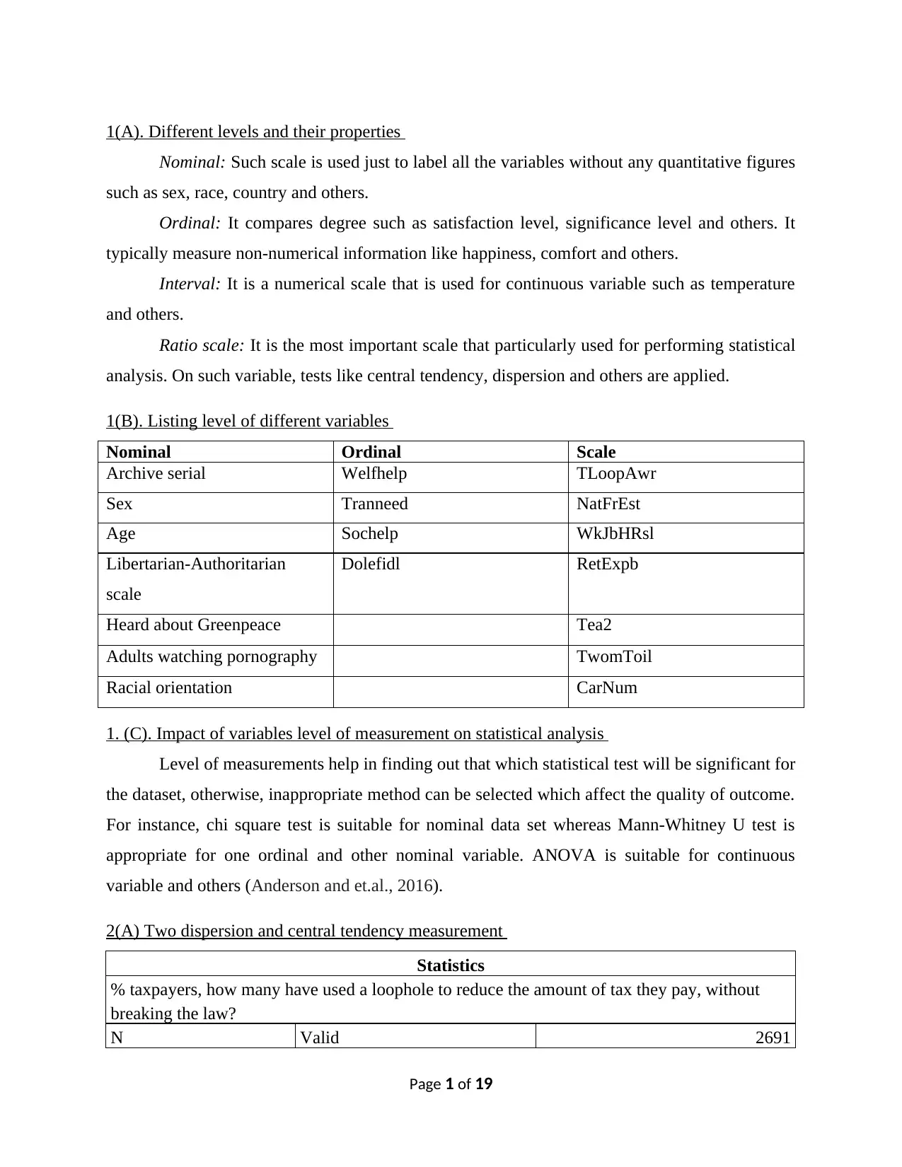
1(A). Different levels and their properties
Nominal: Such scale is used just to label all the variables without any quantitative figures
such as sex, race, country and others.
Ordinal: It compares degree such as satisfaction level, significance level and others. It
typically measure non-numerical information like happiness, comfort and others.
Interval: It is a numerical scale that is used for continuous variable such as temperature
and others.
Ratio scale: It is the most important scale that particularly used for performing statistical
analysis. On such variable, tests like central tendency, dispersion and others are applied.
1(B). Listing level of different variables
Nominal Ordinal Scale
Archive serial Welfhelp TLoopAwr
Sex Tranneed NatFrEst
Age Sochelp WkJbHRsl
Libertarian-Authoritarian
scale
Dolefidl RetExpb
Heard about Greenpeace Tea2
Adults watching pornography TwomToil
Racial orientation CarNum
1. (C). Impact of variables level of measurement on statistical analysis
Level of measurements help in finding out that which statistical test will be significant for
the dataset, otherwise, inappropriate method can be selected which affect the quality of outcome.
For instance, chi square test is suitable for nominal data set whereas Mann-Whitney U test is
appropriate for one ordinal and other nominal variable. ANOVA is suitable for continuous
variable and others (Anderson and et.al., 2016).
2(A) Two dispersion and central tendency measurement
Statistics
% taxpayers, how many have used a loophole to reduce the amount of tax they pay, without
breaking the law?
N Valid 2691
Page 1 of 19
⊘ This is a preview!⊘
Do you want full access?
Subscribe today to unlock all pages.
Trusted by 1+ million students worldwide
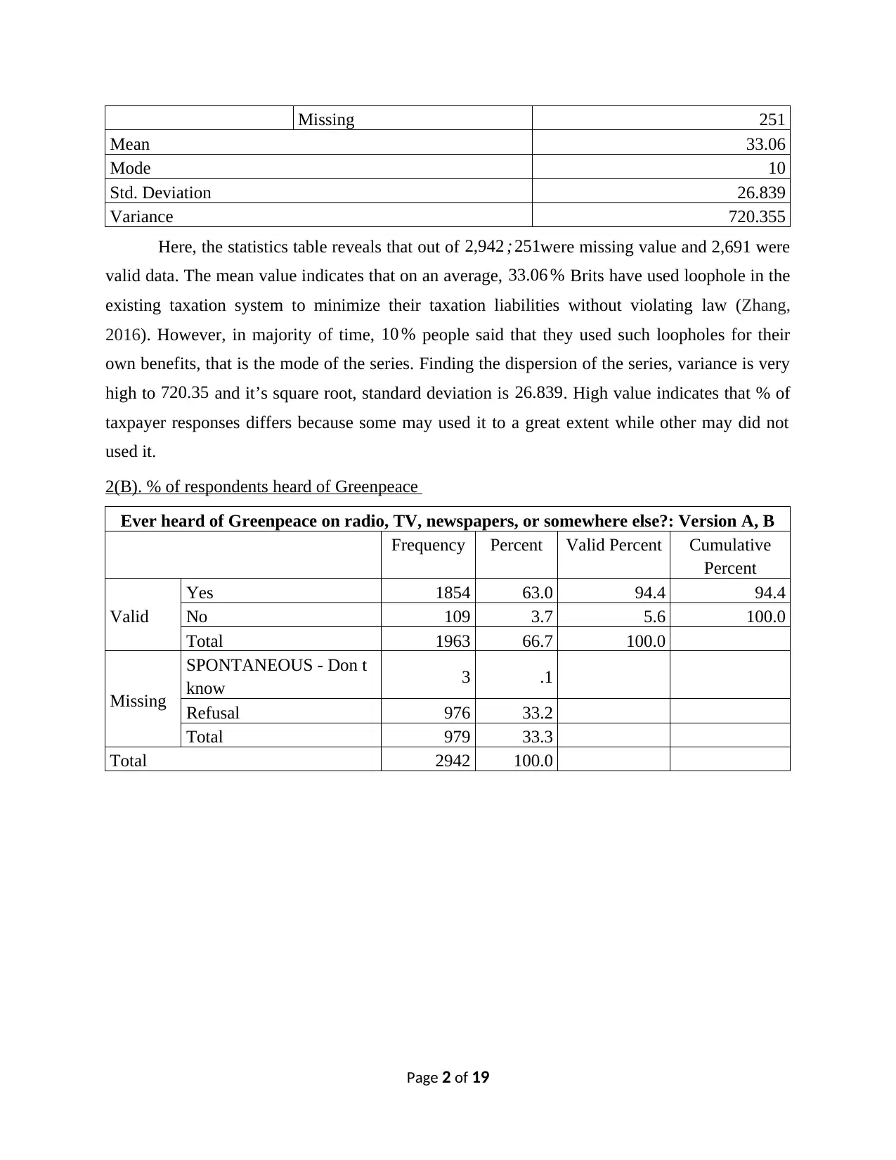
Missing 251
Mean 33.06
Mode 10
Std. Deviation 26.839
Variance 720.355
Here, the statistics table reveals that out of 2,942 ; 251were missing value and 2,691 were
valid data. The mean value indicates that on an average, 33.06 % Brits have used loophole in the
existing taxation system to minimize their taxation liabilities without violating law (Zhang,
2016). However, in majority of time, 10 % people said that they used such loopholes for their
own benefits, that is the mode of the series. Finding the dispersion of the series, variance is very
high to 720.35 and it’s square root, standard deviation is 26.839. High value indicates that % of
taxpayer responses differs because some may used it to a great extent while other may did not
used it.
2(B). % of respondents heard of Greenpeace
Ever heard of Greenpeace on radio, TV, newspapers, or somewhere else?: Version A, B
Frequency Percent Valid Percent Cumulative
Percent
Valid
Yes 1854 63.0 94.4 94.4
No 109 3.7 5.6 100.0
Total 1963 66.7 100.0
Missing
SPONTANEOUS - Don t
know 3 .1
Refusal 976 33.2
Total 979 33.3
Total 2942 100.0
Page 2 of 19
Paraphrase This Document
Need a fresh take? Get an instant paraphrase of this document with our AI Paraphraser
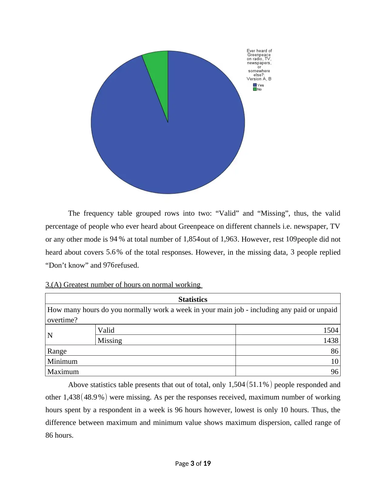
The frequency table grouped rows into two: “Valid” and “Missing”, thus, the valid
percentage of people who ever heard about Greenpeace on different channels i.e. newspaper, TV
or any other mode is 94 % at total number of 1,854out of 1,963. However, rest 109people did not
heard about covers 5.6 % of the total responses. However, in the missing data, 3 people replied
“Don’t know” and 976refused.
3.(A) Greatest number of hours on normal working
Statistics
How many hours do you normally work a week in your main job - including any paid or unpaid
overtime?
N Valid 1504
Missing 1438
Range 86
Minimum 10
Maximum 96
Above statistics table presents that out of total, only 1,504 (51.1% ) people responded and
other 1,438(48.9 %) were missing. As per the responses received, maximum number of working
hours spent by a respondent in a week is 96 hours however, lowest is only 10 hours. Thus, the
difference between maximum and minimum value shows maximum dispersion, called range of
86 hours.
Page 3 of 19
3(B). Recoding to display proportion of percentage working for different time duration
Statistics
Recorded working hours
N Valid 1504
Missing 1438
Recorded working hours
Frequency Percent Valid Percent Cumulative
Percent
Valid
10-20 224 7.6 14.9 14.9
21-40 835 28.4 55.5 70.4
41-60 385 13.1 25.6 96.0
More than 60 60 2.0 4.0 100.0
Total 1504 51.1 100.0
Missing System 1438 48.9
Total 2942 100.0
Page 4 of 19
⊘ This is a preview!⊘
Do you want full access?
Subscribe today to unlock all pages.
Trusted by 1+ million students worldwide
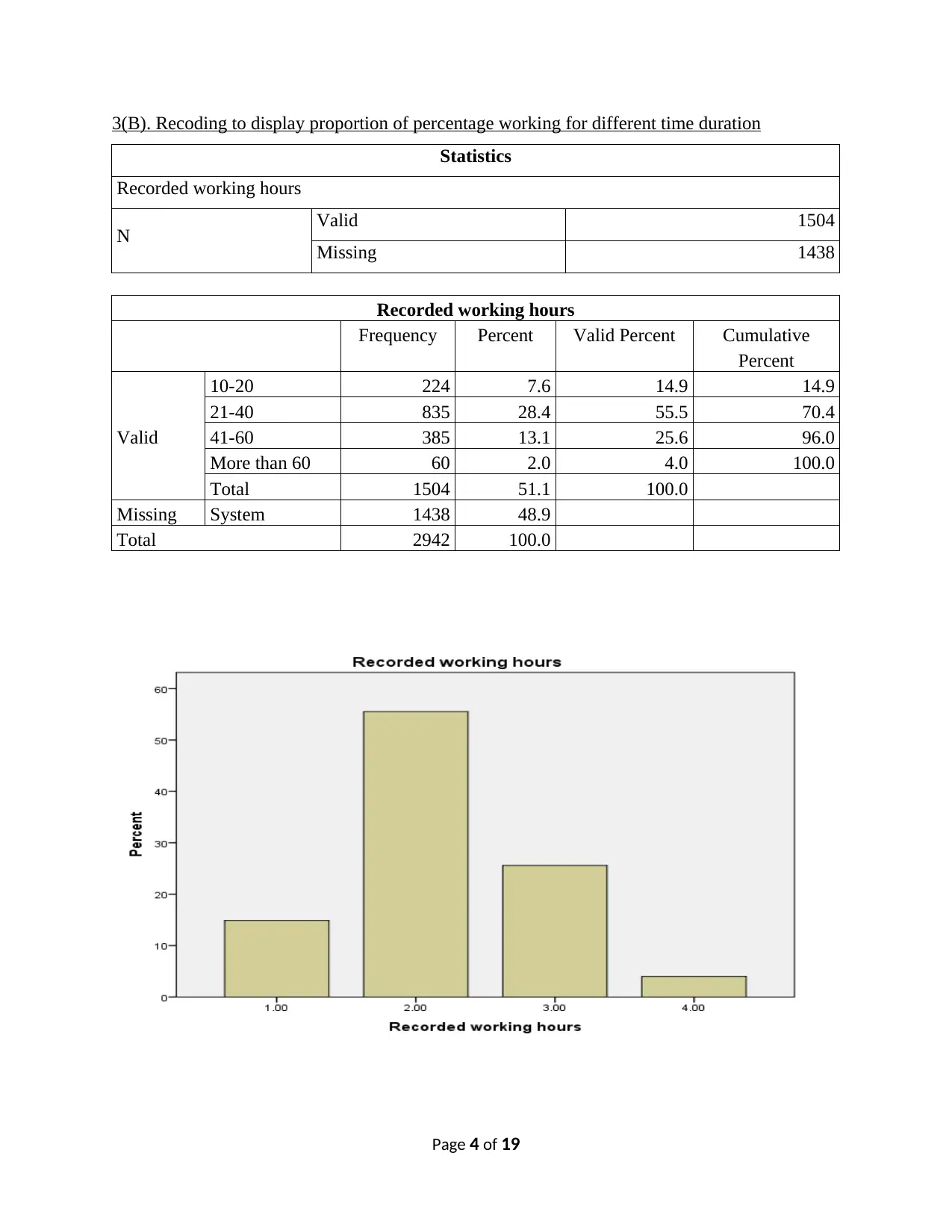
Statistical findings shows that under 10−20 hrs, there are 14.9 % people working.
Maximum number of people works for hours ranging from 21 – 40 hrs with 835 holding 55.5 %
of total valid values whereas 25.6 %=385 member works for 41 – 60 hours in a week. However,
there are only 60 people with 4 % who worked for a long duration of 61 hours or more.
3.(C). % of respondents strongly agreeing across people working more than 60 hours
Statisticsa
The welfare state encourages people to stop helping each other
N Valid 48
Missing 12
a. Recorded working hours = More than 60
The welfare state encourages people to stop helping each othera
Frequency Percent Valid Percent Cumulative
Percent
Valid
Agree strongly 4 6.7 8.3 8.3
Agree 18 30.0 37.5 45.8
Neither agree nor disagree 13 21.7 27.1 72.9
Disagree 10 16.7 20.8 93.8
Disagree strongly 3 5.0 6.3 100.0
Total 48 80.0 100.0
Missing skip, didn't return SC
questionnaire 12 20.0
Total 60 100.0
a. Recorded working hours = More than 60
Page 5 of 19
Paraphrase This Document
Need a fresh take? Get an instant paraphrase of this document with our AI Paraphraser
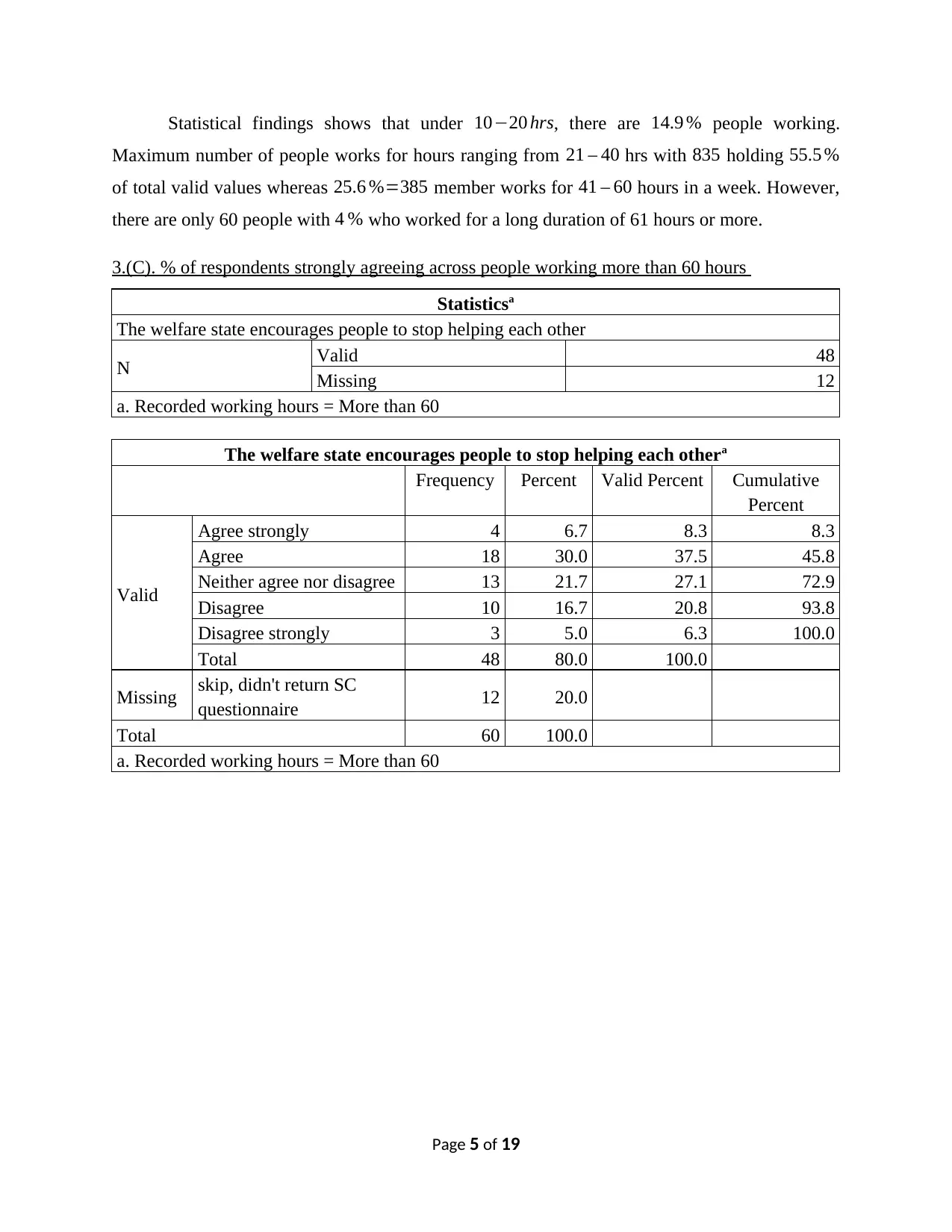
In total, there are60 members, out of this, only 48 members responded that whether
welfare state encourages people to stop helping each other or not and rest 12 were missing data.
Out of 48, there are four (8.3 %) members who strongly agree with this and said that there is no
doubt, that welfare state in the country will definitely motivate all the members to not to help
each other.
4 (A). Confidence interval for the men age of retiring
Case Processing Summary
Cases
Valid Missing Total
N Percent N Percent N Percent
At what age do you expect
to retire from your main
job?
1051 35.7% 1891 64.3% 2942 100.0%
Page 6 of 19
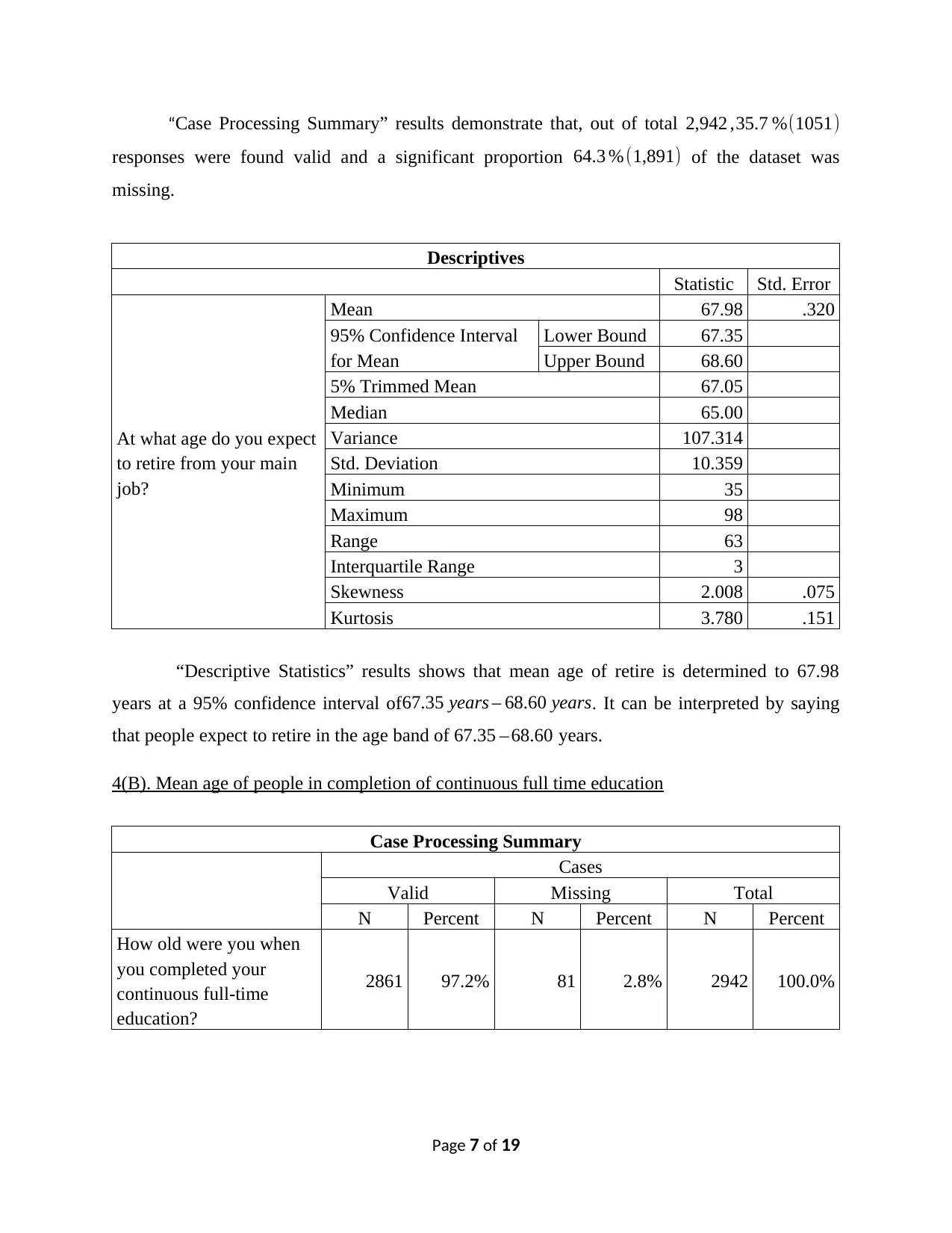
“Case Processing Summary” results demonstrate that, out of total 2,942 ,35.7 %(1051)
responses were found valid and a significant proportion 64.3 % (1,891) of the dataset was
missing.
Descriptives
Statistic Std. Error
At what age do you expect
to retire from your main
job?
Mean 67.98 .320
95% Confidence Interval
for Mean
Lower Bound 67.35
Upper Bound 68.60
5% Trimmed Mean 67.05
Median 65.00
Variance 107.314
Std. Deviation 10.359
Minimum 35
Maximum 98
Range 63
Interquartile Range 3
Skewness 2.008 .075
Kurtosis 3.780 .151
“Descriptive Statistics” results shows that mean age of retire is determined to 67.98
years at a 95% confidence interval of 67.35 years – 68.60 years. It can be interpreted by saying
that people expect to retire in the age band of 67.35 – 68.60 years.
4(B). Mean age of people in completion of continuous full time education
Case Processing Summary
Cases
Valid Missing Total
N Percent N Percent N Percent
How old were you when
you completed your
continuous full-time
education?
2861 97.2% 81 2.8% 2942 100.0%
Page 7 of 19
⊘ This is a preview!⊘
Do you want full access?
Subscribe today to unlock all pages.
Trusted by 1+ million students worldwide
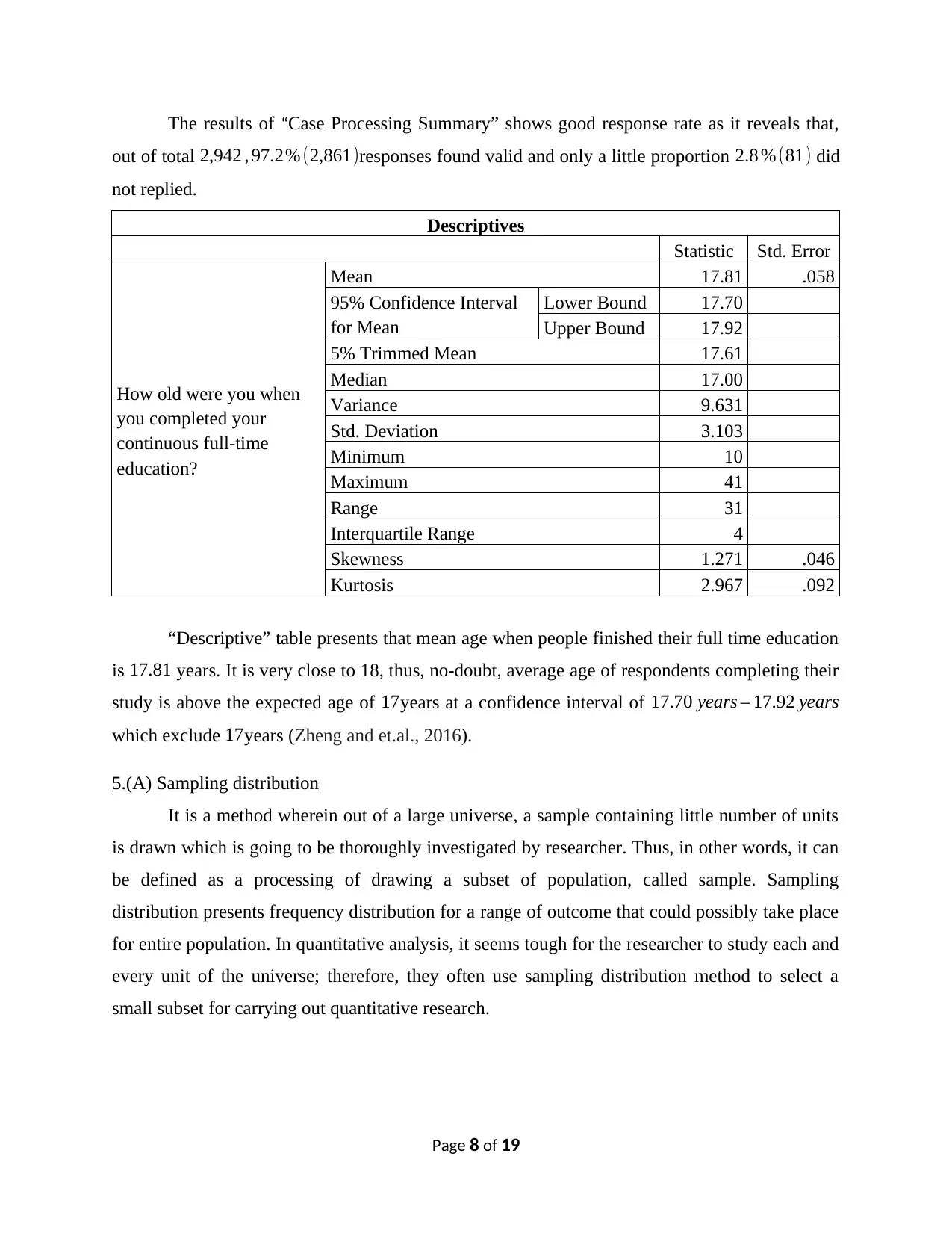
The results of “Case Processing Summary” shows good response rate as it reveals that,
out of total 2,942 , 97.2% (2,861)responses found valid and only a little proportion 2.8 %(81) did
not replied.
Descriptives
Statistic Std. Error
How old were you when
you completed your
continuous full-time
education?
Mean 17.81 .058
95% Confidence Interval
for Mean
Lower Bound 17.70
Upper Bound 17.92
5% Trimmed Mean 17.61
Median 17.00
Variance 9.631
Std. Deviation 3.103
Minimum 10
Maximum 41
Range 31
Interquartile Range 4
Skewness 1.271 .046
Kurtosis 2.967 .092
“Descriptive” table presents that mean age when people finished their full time education
is 17.81 years. It is very close to 18, thus, no-doubt, average age of respondents completing their
study is above the expected age of 17years at a confidence interval of 17.70 years – 17.92 years
which exclude 17years (Zheng and et.al., 2016).
5.(A) Sampling distribution
It is a method wherein out of a large universe, a sample containing little number of units
is drawn which is going to be thoroughly investigated by researcher. Thus, in other words, it can
be defined as a processing of drawing a subset of population, called sample. Sampling
distribution presents frequency distribution for a range of outcome that could possibly take place
for entire population. In quantitative analysis, it seems tough for the researcher to study each and
every unit of the universe; therefore, they often use sampling distribution method to select a
small subset for carrying out quantitative research.
Page 8 of 19
Paraphrase This Document
Need a fresh take? Get an instant paraphrase of this document with our AI Paraphraser
5. (B). Role of sampling in statistical inference
Sampling distribution plays an important role in drawing statistical inferences about the
population. It is because; statistical inferences drawn through studying the sample are based on
probability of something, which enable investigator to infer interesting facts and findings about
the given population (Field, 2013). Here, in order to assure the validity and reliability of the
analysis about the entire population, a careful attention needs to be paid on selection of a highly
representative sample for the universe, so that, results can be applied to the entire universe.
Random selection method is found appropriate because it is biasfree and helps to select a
representative sample.
6.(A). Impact of sex over transgender people’s belief
H0: A Transgender person undergone through this process due to very superficial and temporary
need is irrelevant to their sex.
H1: Transgender people undergone through this process due to very superficial and temporary
need depend on their sex.
Test: ANOVA
Test statistics: 0.05 or 5%
Model Summary
Model R R Square Adjusted R Square Std. Error of the
Estimate
1 .166a .028 .027 1.071
a. Predictors: (Constant), Person 1 SEX
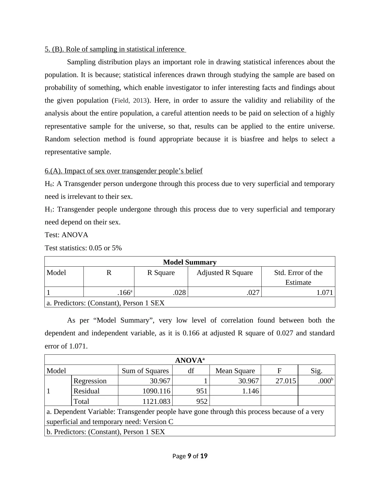
As per “Model Summary”, very low level of correlation found between both the
dependent and independent variable, as it is 0.166 at adjusted R square of 0.027 and standard
error of 1.071.
ANOVAa
Model Sum of Squares df Mean Square F Sig.
1
Regression 30.967 1 30.967 27.015 .000b
Residual 1090.116 951 1.146
Total 1121.083 952
a. Dependent Variable: Transgender people have gone through this process because of a very
superficial and temporary need: Version C
b. Predictors: (Constant), Person 1 SEX
Page 9 of 19
Sampling distribution plays an important role in drawing statistical inferences about the
population. It is because; statistical inferences drawn through studying the sample are based on
probability of something, which enable investigator to infer interesting facts and findings about
the given population (Field, 2013). Here, in order to assure the validity and reliability of the
analysis about the entire population, a careful attention needs to be paid on selection of a highly
representative sample for the universe, so that, results can be applied to the entire universe.
Random selection method is found appropriate because it is biasfree and helps to select a
representative sample.
6.(A). Impact of sex over transgender people’s belief
H0: A Transgender person undergone through this process due to very superficial and temporary
need is irrelevant to their sex.
H1: Transgender people undergone through this process due to very superficial and temporary
need depend on their sex.
Test: ANOVA
Test statistics: 0.05 or 5%
Model Summary
Model R R Square Adjusted R Square Std. Error of the
Estimate
1 .166a .028 .027 1.071
a. Predictors: (Constant), Person 1 SEX
As per “Model Summary”, very low level of correlation found between both the
dependent and independent variable, as it is 0.166 at adjusted R square of 0.027 and standard
error of 1.071.
ANOVAa
Model Sum of Squares df Mean Square F Sig.
1
Regression 30.967 1 30.967 27.015 .000b
Residual 1090.116 951 1.146
Total 1121.083 952
a. Dependent Variable: Transgender people have gone through this process because of a very
superficial and temporary need: Version C
b. Predictors: (Constant), Person 1 SEX
Page 9 of 19
Coefficientsa
Model Unstandardized Coefficients Standardized
Coefficients
t Sig.
B Std. Error Beta
1 (Constant) 3.317 .116 28.593 .000
Person 1 SEX .365 .070 .166 5.198 .000
a. Dependent Variable: Transgender people have gone through this process because of a very
superficial and temporary need: Version C
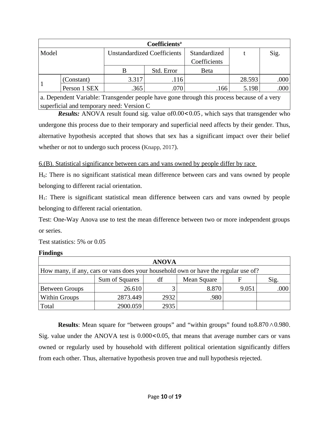
Results: ANOVA result found sig. value of 0.00<0.05 , which says that transgender who
undergone this process due to their temporary and superficial need affects by their gender. Thus,
alternative hypothesis accepted that shows that sex has a significant impact over their belief
whether or not to undergo such process (Knapp, 2017).
6.(B). Statistical significance between cars and vans owned by people differ by race
H0: There is no significant statistical mean difference between cars and vans owned by people
belonging to different racial orientation.
H1: There is significant statistical mean difference between cars and vans owned by people
belonging to different racial orientation.
Test: One-Way Anova use to test the mean difference between two or more independent groups
or series.
Test statistics: 5% or 0.05
Findings
ANOVA
How many, if any, cars or vans does your household own or have the regular use of?
Sum of Squares df Mean Square F Sig.
Between Groups 26.610 3 8.870 9.051 .000
Within Groups 2873.449 2932 .980
Total 2900.059 2935
Results: Mean square for “between groups” and “within groups” found to8.870∧0.980.
Sig. value under the ANOVA test is 0.000< 0.05, that means that average number cars or vans
owned or regularly used by household with different political orientation significantly differs
from each other. Thus, alternative hypothesis proven true and null hypothesis rejected.
Page 10 of 19
Model Unstandardized Coefficients Standardized
Coefficients
t Sig.
B Std. Error Beta
1 (Constant) 3.317 .116 28.593 .000
Person 1 SEX .365 .070 .166 5.198 .000
a. Dependent Variable: Transgender people have gone through this process because of a very
superficial and temporary need: Version C
Results: ANOVA result found sig. value of 0.00<0.05 , which says that transgender who
undergone this process due to their temporary and superficial need affects by their gender. Thus,
alternative hypothesis accepted that shows that sex has a significant impact over their belief
whether or not to undergo such process (Knapp, 2017).
6.(B). Statistical significance between cars and vans owned by people differ by race
H0: There is no significant statistical mean difference between cars and vans owned by people
belonging to different racial orientation.
H1: There is significant statistical mean difference between cars and vans owned by people
belonging to different racial orientation.
Test: One-Way Anova use to test the mean difference between two or more independent groups
or series.
Test statistics: 5% or 0.05
Findings
ANOVA
How many, if any, cars or vans does your household own or have the regular use of?
Sum of Squares df Mean Square F Sig.
Between Groups 26.610 3 8.870 9.051 .000
Within Groups 2873.449 2932 .980
Total 2900.059 2935
Results: Mean square for “between groups” and “within groups” found to8.870∧0.980.
Sig. value under the ANOVA test is 0.000< 0.05, that means that average number cars or vans
owned or regularly used by household with different political orientation significantly differs
from each other. Thus, alternative hypothesis proven true and null hypothesis rejected.
Page 10 of 19
⊘ This is a preview!⊘
Do you want full access?
Subscribe today to unlock all pages.
Trusted by 1+ million students worldwide
1 out of 19
Related Documents


Your All-in-One AI-Powered Toolkit for Academic Success.
+13062052269
info@desklib.com
Available 24*7 on WhatsApp / Email
![[object Object]](/_next/static/media/star-bottom.7253800d.svg)
Unlock your academic potential
Copyright © 2020–2026 A2Z Services. All Rights Reserved. Developed and managed by ZUCOL.