University of Australia: CIVE 5015 Assignment 1 Report, SP2 2018

This report details a student's application of data analysis techniques using SPSS. It begins with descriptive analysis, including frequency analysis, histograms, and boxplots to explore the dataset of annual rainfall, annual daily maximum rainfall, and annual monthly maximum rainfall. The report then covers data recoding to create categorical variables, followed by a Chi-square test to assess the association between annual rainfall and annual daily maximum rainfall. Further analysis includes t-tests to compare means of two groups and ANOVA for comparing means of more than two groups. The methodology, results, and discussion for each task are presented, providing a comprehensive overview of the data analysis process. The student utilizes data from the Australian Bureau of Meteorology and applies various statistical methods to draw conclusions about the rainfall data. The report provides a detailed analysis of the data using SPSS software, including data collection, variable configuration, and the interpretation of results from various statistical tests.

Assignment 1: Tutorial Questions
CIVE 5015
Research Data Analysis
SP2 2018
University of Australia
Dataset:
Annual rainfall, Annual daily maximum rainfall, Annual monthly maximum rainfall
Name:
Student ID:
1

Table of Contents
1. Introduction..............................................................................................................................4
2. SPSS version 25 data analysis..................................................................................................4
2.1 Task 1: Descriptive analysis.............................................................................................4
2.1.1 Methodology..............................................................................................................5
2.1.2 Results........................................................................................................................6
2.1.2.1 Descriptive analysis...................................................................................................6
2.1.2.2 Histogram for annual rainfall (AR) with Distribution Curve....................................7
2.1.2.3 Histogram for annual daily maximum rainfall (ADMR) with Distribution Curve. . .7
2.1.2.4 Histogram for annual monthly maximum rainfall (AMMR) with Distribution Curve
8
2.1.2.5 Boxplots.....................................................................................................................8
2.1.3 Discussion..................................................................................................................8
2.2 Task 2: Data Recoding......................................................................................................9
2.2.2 Results......................................................................................................................10
2.2.2.1 Data Analysis...........................................................................................................10
2.2.2.2 Data recoding...........................................................................................................10
2.2.3 Summary..................................................................................................................11
2.3 Task 3: Chi square Test...................................................................................................11
2.3.2 Results......................................................................................................................11
2

2.3.2.1 Establish Chi Square Test Hypothesis.....................................................................11
2.3.2.2 Chi-Square output....................................................................................................12
2.3.3 Discussion................................................................................................................13
2.4 Task 4: T-test..................................................................................................................13
2.4.1 Methodology............................................................................................................14
2.4.2 Results......................................................................................................................14
2.4.2.1 Establish T- Test Hypothesis...................................................................................14
2.4.2.2 T-test output.............................................................................................................15
2.4.3 Discussion................................................................................................................15
2.5 Task 5: ANOVA.............................................................................................................16
2.5.1 Methodology............................................................................................................16
2.5.2 Results......................................................................................................................16
2.5.2.1 Establish ANOVA Test Hypothesis........................................................................16
2.5.2.2 ANOVA output........................................................................................................17
2.5.3 Discussion................................................................................................................18
3. Conclusion..............................................................................................................................18
References......................................................................................................................................19
Appendixes....................................................................................................................................20
3

1. Introduction
This study is applying the data analysis skills which is a component of the research. The IBM
Statistical Software for Social Sciences (SPSS) is used to perform the required analysis of the
given data set. According to Levesque (2007), SPSS is a powerful software that can be used to
perform various analysis ranging from comparing of means to reliability testing among many
others. The software has syntax part and the point and click sections where people can use to
perform various analysis. It is easy to use and very friendly to even non-statisticians. This study
utilized the dataset on Annual rainfall (AR), Annual daily maximum rainfall (ADMR), Annual
monthly maximum rainfall (AMMR). The aim of the study is to demonstrate the data analysis
skills and apply them on real life events.
2. SPSS version 25 data analysis
This section is divided into 5 different subsections that explains the utilization of different SPSS
techniques to perform analysis. Data for this study was collected from the following website
www.bom.gov.au. The next sections outlines the step-by-step used to perform the various
analysis. The SPSS output and results have also been provided along with the interpretation of
the various results. The preliminary analysis which tries to explore the dataset is the first
subsection. Other analysis techniques discussed in this report include the Chi-square test of
association, t-test for comparing means of two factors, analysis of variance (ANOVA) for
comparing means of more than 2 factors.
2.1 Task 1: Descriptive analysis
Descriptive analysis which also includes frequency analysis is the most commonly used analysis
for exploring the dataset before performing any inferential analysis. The analysis captures the
4

mean, mode and median of the data set commonly known as the measures of central tendency.
Other measures include the standard deviation which is a measure of variation. To check for
distribution of data, kurtosis and skewness was used.
2.1.1 Methodology
This section presents the methodology used from data collection to presentation of the analyzed
data set.
5
1. Data collection
Computing the rainfall data into Microsoft Excel documents
Access Bom website > Select the station > Download the data sets > Tabulate the data
into Microsoft Excel
2. Data entries
Extract water consumption data to the SPSS software. Once the data has been extracted
into the software, configure the variables to scale measure.
Extract Excel water consumption data into SPSS variable name > Change the name
and the scale measure for the variable.
3. SPSS function: Descriptive Analysis
The next step is to perform the descriptive analysis for the three variables. The analysis
seeks to produce the mean, median and mode.
Open SPSS file > Analyze > Descriptive Statistics > Frequencies & Descriptive

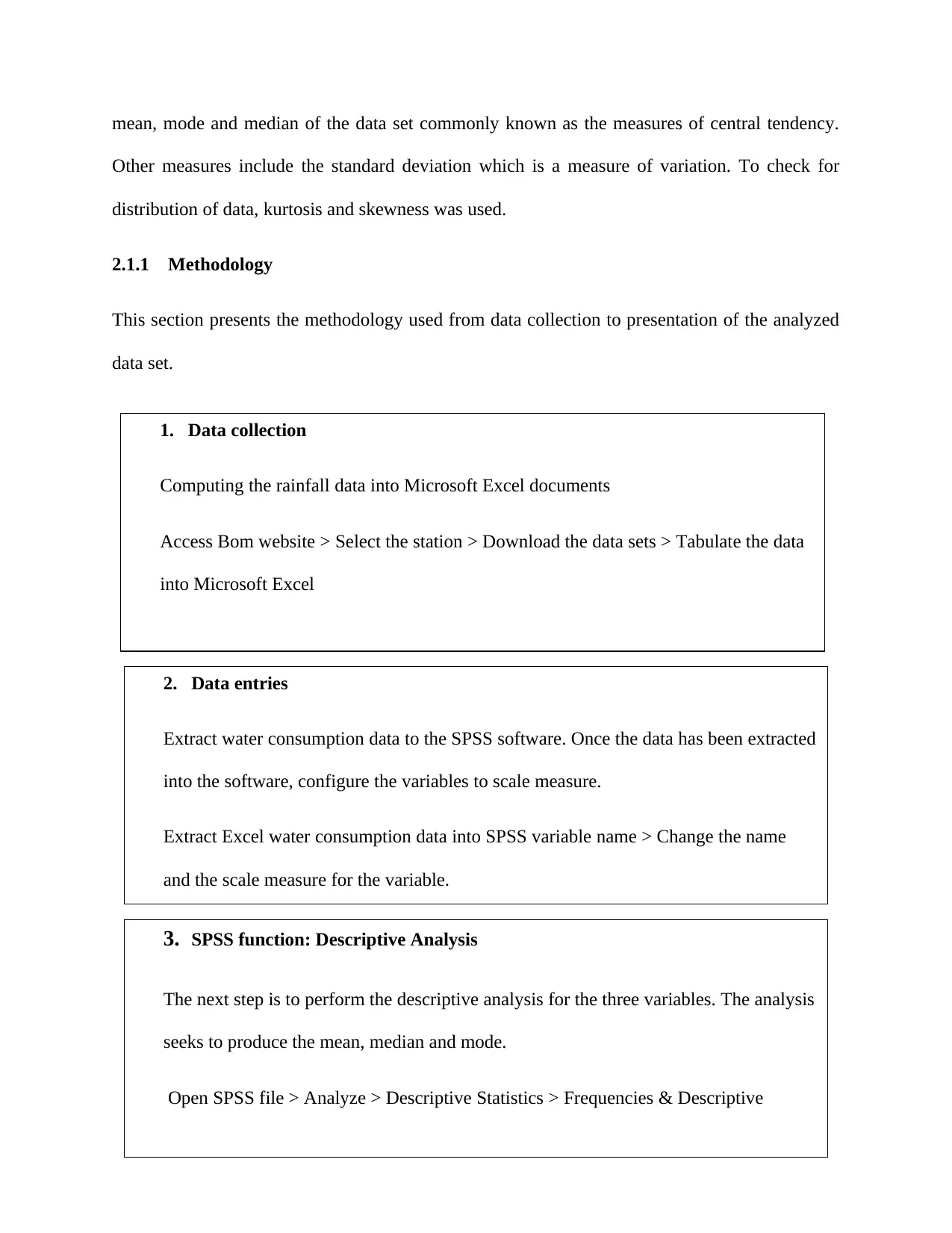
2.1.2 Results
2.1.2.1 Descriptive analysis
YEAR AR ADMR MADM AMMR MAMM NO25
R R
N Valid 30 30 30 30 30 30 30
Missing 0 0 0 0 0 0 0
Mean 2003.50 442.770 33.757 6.30 87.083 6.70 2.00
Median 2003.50 440.550 29.650 6.00 87.000 7.00 2.00
Mode 1989a 266.9a 11.2a 9 42.2a 7 2
Std. Deviation 8.803 91.6525 17.7444 3.687 21.4501 2.037 1.531
Skewness .000 .254 1.690 .129 -.096 -.481 1.111
Std. Error
of .427 .427 .427 .427 .427 .427 .427
Skewness
Kurtosis -1.200 .135 2.669 -1.276 -.739 -.237 1.446
Std. Error of
Kurtosis .833 .833 .833 .833 .833 .833 .833
6
4. SPSS function: Visualizing Data (Drawing Histograms and Boxplots)
The last step was to construct visualization plots (boxplots and histograms) for the
three variables. The steps are;
Open SPSS file > Graphs > Legacy dialogs > Boxplots
Open SPSS file > Graphs > Legacy dialogs > Histograms
N Minimum Maximum Mean
Std.
Deviation
YEAR 30 1989 2018 2003.50 8.803
AR 30 266.9 645.7 442.770 91.6525
ADMR 30 11.2 87.8 33.757 17.7444
MADMR 30 1 12 6.30 3.687
AMMR 30 42.2 125.8 87.083 21.4501
MAMMR 30 2 10 6.70 2.037
NO25 30 0 6 2.00 1.531
Valid N
(listwise) 30

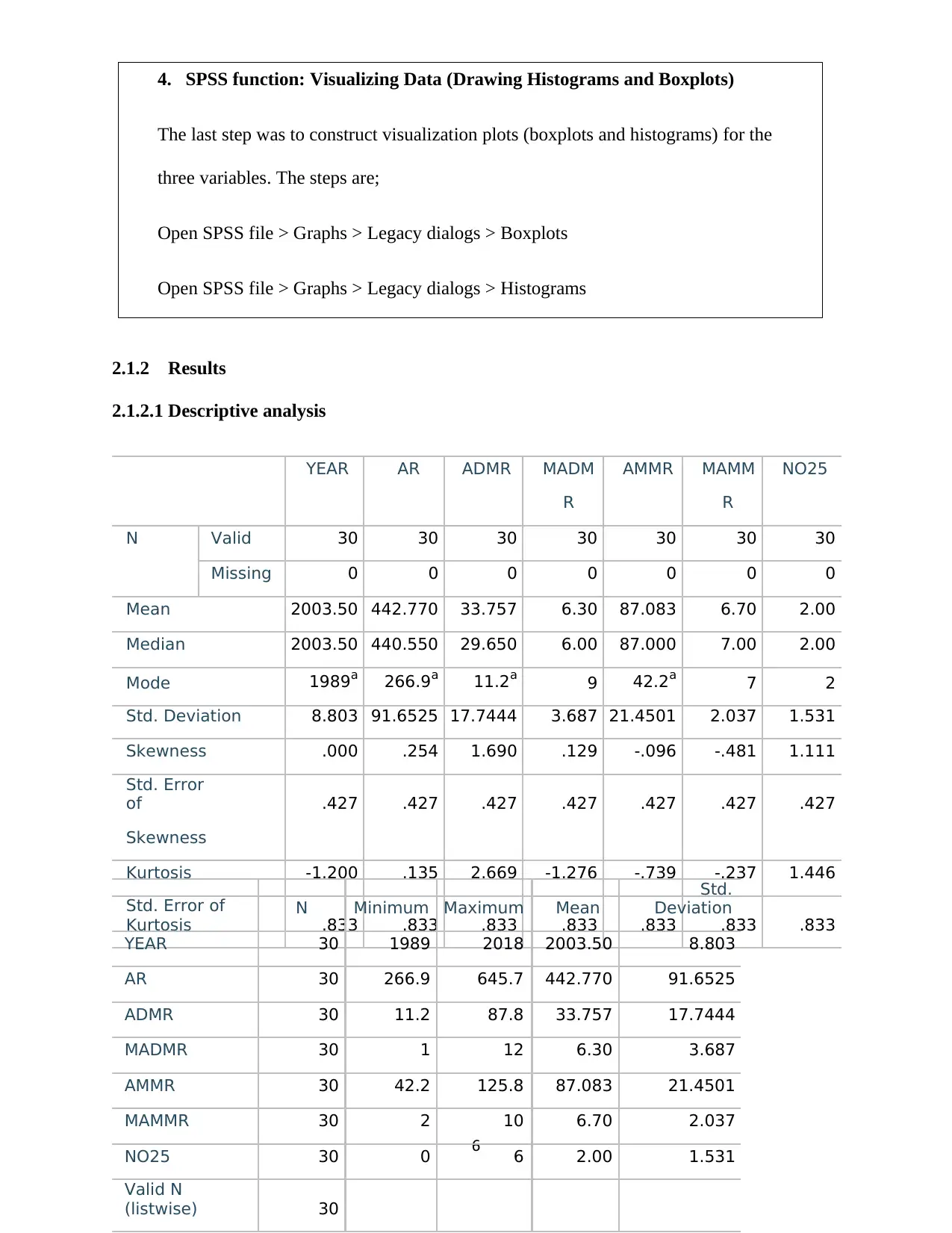
2.1.2.2 Histogram for annual rainfall (AR) with Distribution Curve
2.1.2.3 Histogram for annual daily maximum rainfall (ADMR) with Distribution Curve
2.1.2.4 Histogram for annual monthly maximum rainfall (AMMR) with Distribution Curve
7

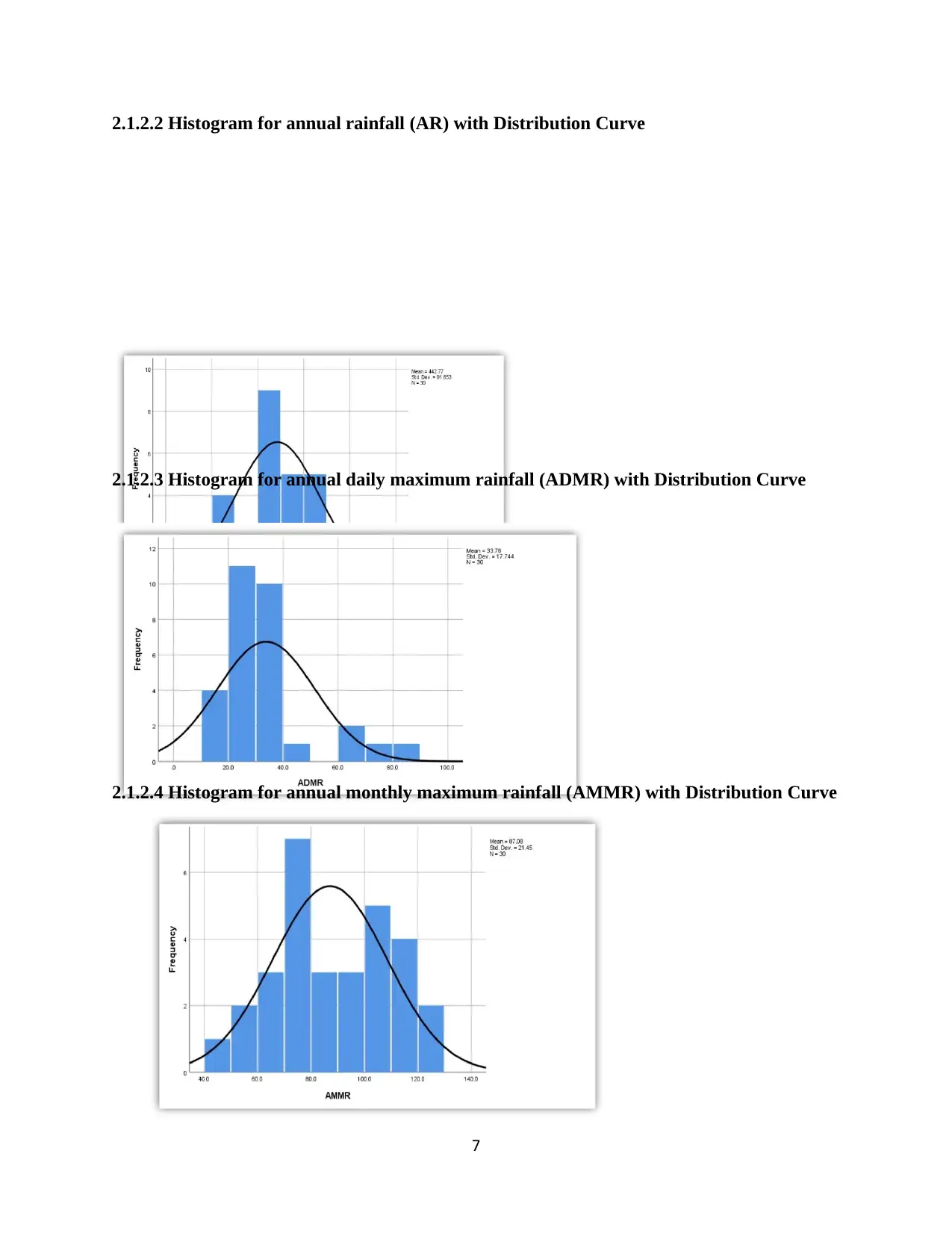
2.1.2.5 Boxplots
2.1.3 Discussion
Sections 2.1.2.1 – 2.1.2.5 presents the results of the descriptive analysis as well as the plots for
the different variables (annual rainfall, annual daily maximum rainfall and the annual monthly
maximum rainfall). As can be seen from the table, annual rainfall had the highest mean (M =
442.77, SD = 91.65) while annual daily maximum rainfall had the lowest mean (M = 33.76, SD
= 17.74). The annual monthly maximum rainfall had an average of 87.08 (SD = 21.45). In terms
of skewness, annual monthly maximum rainfall was the least skewed (skewness = -.096) while
annual daily maximum rainfall (ADMR) had the highest skewness value (skewness = 1.690).
The values further shows that the data for annual monthly maximum rainfall (AMMR) and
annual rainfall were found to be close to normal distribution while that of annual daily maximum
rainfall is highly positively skewed.
8

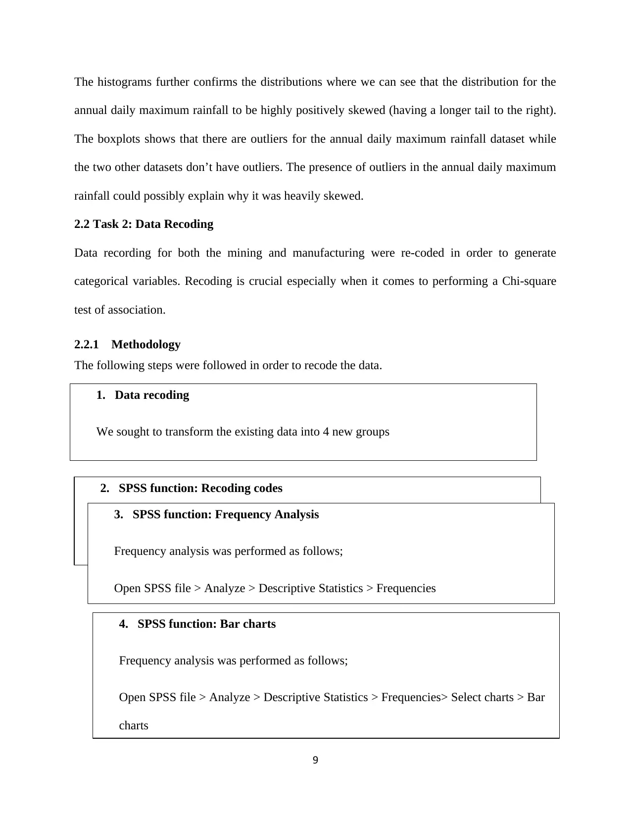
The histograms further confirms the distributions where we can see that the distribution for the
annual daily maximum rainfall to be highly positively skewed (having a longer tail to the right).
The boxplots shows that there are outliers for the annual daily maximum rainfall dataset while
the two other datasets don’t have outliers. The presence of outliers in the annual daily maximum
rainfall could possibly explain why it was heavily skewed.
2.2 Task 2: Data Recoding
Data recording for both the mining and manufacturing were re-coded in order to generate
categorical variables. Recoding is crucial especially when it comes to performing a Chi-square
test of association.
2.2.1 Methodology
The following steps were followed in order to recode the data.
9
1. Data recoding
We sought to transform the existing data into 4 new groups
2. SPSS function: Recoding codes
We sought to transform the existing data into 4 new groups. The codes are given
below;
3. SPSS function: Frequency Analysis
Frequency analysis was performed as follows;
Open SPSS file > Analyze > Descriptive Statistics > Frequencies
4. SPSS function: Bar charts
Frequency analysis was performed as follows;
Open SPSS file > Analyze > Descriptive Statistics > Frequencies> Select charts > Bar
charts

2.2.2 Results
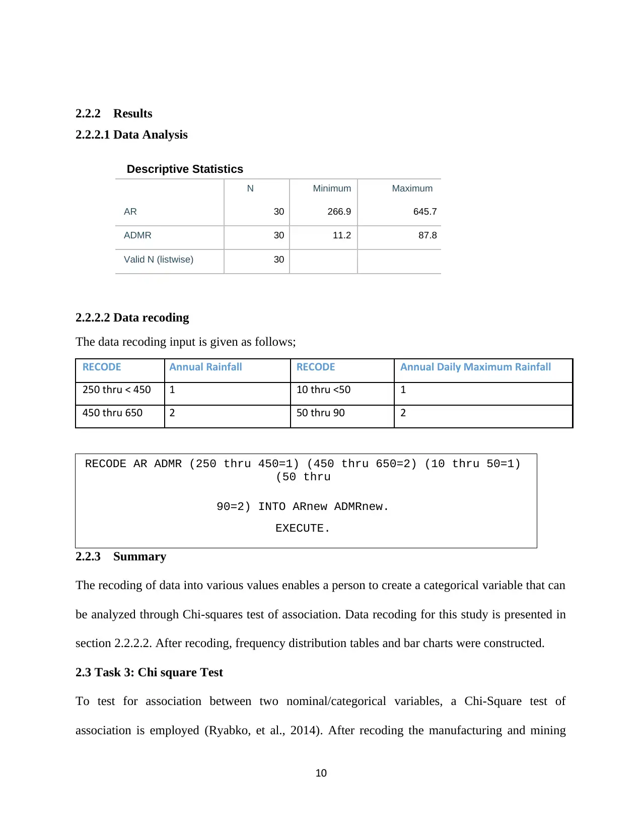
2.2.2.1 Data Analysis
Descriptive Statistics
2.2.2.2 Data recoding
The data recoding input is given as follows;
RECODE Annual Rainfall RECODE Annual Daily Maximum Rainfall
250 thru < 450 1 10 thru <50 1
450 thru 650 2 50 thru 90 2
2.2.3 Summary
The recoding of data into various values enables a person to create a categorical variable that can
be analyzed through Chi-squares test of association. Data recoding for this study is presented in
section 2.2.2.2. After recoding, frequency distribution tables and bar charts were constructed.
2.3 Task 3: Chi square Test
To test for association between two nominal/categorical variables, a Chi-Square test of
association is employed (Ryabko, et al., 2014). After recoding the manufacturing and mining
10
RECODE AR ADMR (250 thru 450=1) (450 thru 650=2) (10 thru 50=1)
(50 thru
90=2) INTO ARnew ADMRnew.
EXECUTE.
N Minimum Maximum
AR 30 266.9 645.7
ADMR 30 11.2 87.8
Valid N (listwise) 30

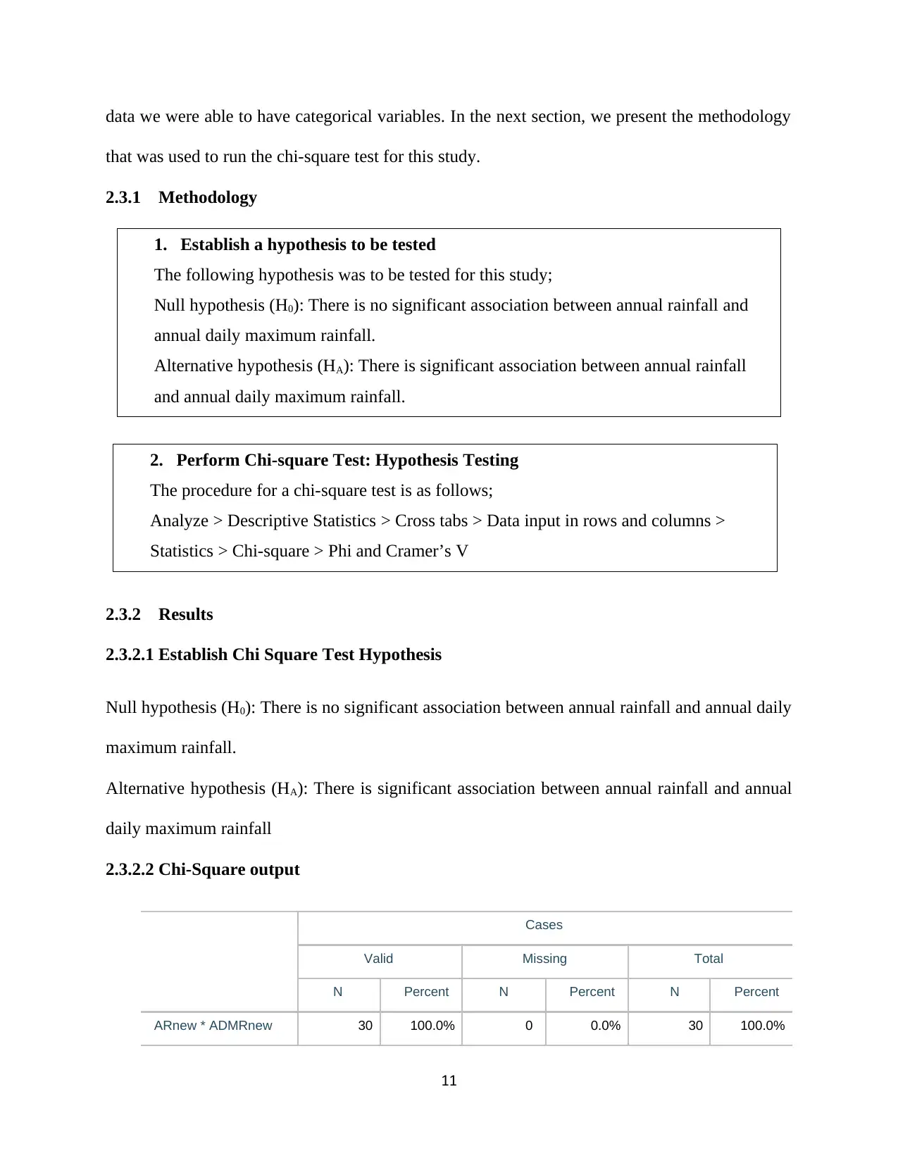
data we were able to have categorical variables. In the next section, we present the methodology
that was used to run the chi-square test for this study.
2.3.1 Methodology
2.3.2 Results
2.3.2.1 Establish Chi Square Test Hypothesis
Null hypothesis (H0): There is no significant association between annual rainfall and annual daily
maximum rainfall.
Alternative hypothesis (HA): There is significant association between annual rainfall and annual
daily maximum rainfall
2.3.2.2 Chi-Square output
Cases
Valid Missing Total
N Percent N Percent N Percent
ARnew * ADMRnew 30 100.0% 0 0.0% 30 100.0%
11
1. Establish a hypothesis to be tested
The following hypothesis was to be tested for this study;
Null hypothesis (H0): There is no significant association between annual rainfall and
annual daily maximum rainfall.
Alternative hypothesis (HA): There is significant association between annual rainfall
and annual daily maximum rainfall.
2. Perform Chi-square Test: Hypothesis Testing
The procedure for a chi-square test is as follows;
Analyze > Descriptive Statistics > Cross tabs > Data input in rows and columns >
Statistics > Chi-square > Phi and Cramer’s V

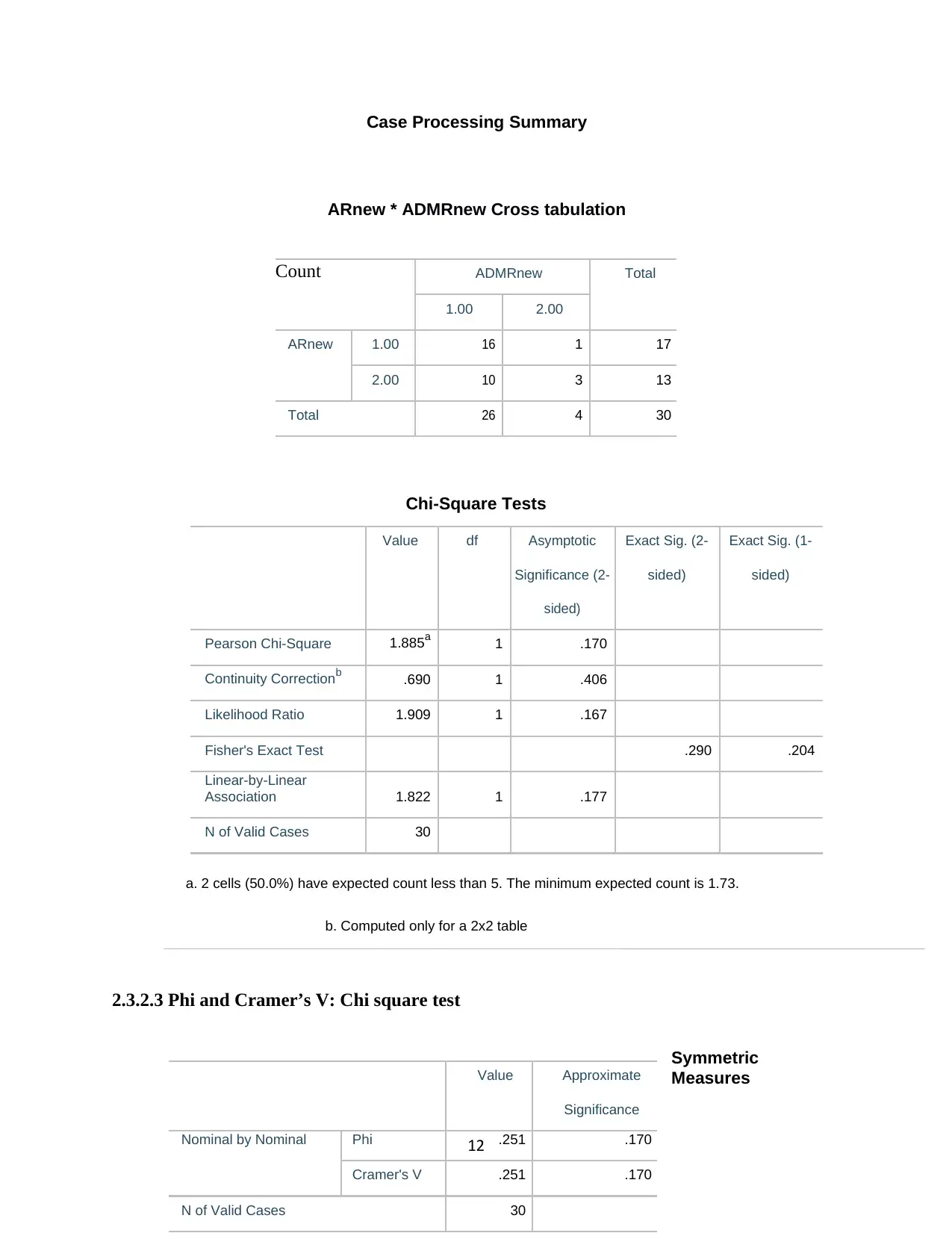
Case Processing Summary
ARnew * ADMRnew Cross tabulation
Chi-Square Tests
Value df Asymptotic Exact Sig. (2- Exact Sig. (1-
Significance (2- sided) sided)
sided)
Pearson Chi-Square 1.885a 1 .170
Continuity Correctionb .690 1 .406
Likelihood Ratio 1.909 1 .167
Fisher's Exact Test .290 .204
Linear-by-Linear
Association 1.822 1 .177
N of Valid Cases 30
a. 2 cells (50.0%) have expected count less than 5. The minimum expected count is 1.73.
b. Computed only for a 2x2 table
2.3.2.3 Phi and Cramer’s V: Chi square test
Symmetric
Measures
12
Count ADMRnew Total
1.00 2.00
ARnew 1.00 16 1 17
2.00 10 3 13
Total 26 4 30
Value Approximate
Significance
Nominal by Nominal Phi .251 .170
Cramer's V .251 .170
N of Valid Cases 30