SPSS Assignment: Data Analysis, Hypothesis Testing and Regression

This SPSS assignment solution provides a detailed analysis of various statistical methods. It includes univariate descriptive statistics for residency duration, cross-tabulation to explore the association between gender and EU enlargement opinions (controlling for government approval), independent samples t-tests to compare residency years between genders, and ANOVA to assess differences in residency length across nationalities. It also covers multiple regression analysis to predict residency years based on education, religiosity, and standard of living. The document presents the hypotheses tested, the statistical results (including p-values and significance levels), and interpretations of the findings. The assignment uses SPSS to perform the analyses and interpret the output, offering insights into the relationships between different variables within the dataset.

Running Head: SPSS ASSIGNMENT 1
SPSS Assignment
Name:
Institution:
19th May 2018

SPSS ASSIGNMENT 2
Univariate descriptive statistics
In this section, we sought to provide the descriptive statistics for the period of residency.
Respondents were asked to state how long (in years) they have been living in their current
residential community.
The variable selected is a numerical variable which required respondents to respond by stating
the years they have lived.
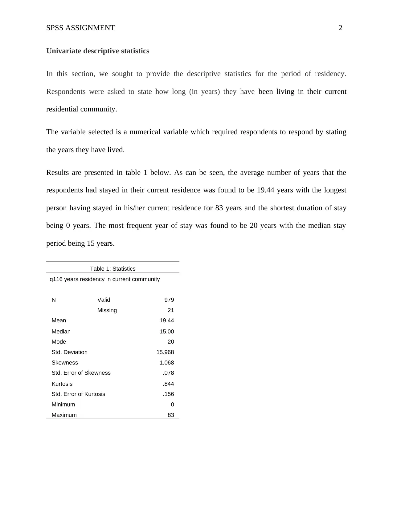
Results are presented in table 1 below. As can be seen, the average number of years that the
respondents had stayed in their current residence was found to be 19.44 years with the longest
person having stayed in his/her current residence for 83 years and the shortest duration of stay
being 0 years. The most frequent year of stay was found to be 20 years with the median stay
period being 15 years.
Table 1: Statistics
q116 years residency in current community
N Valid 979
Missing 21
Mean 19.44
Median 15.00
Mode 20
Std. Deviation 15.968
Skewness 1.068
Std. Error of Skewness .078
Kurtosis .844
Std. Error of Kurtosis .156
Minimum 0
Maximum 83

SPSS ASSIGNMENT 3
Cross-tabulation
For this section, the aim was to find out whether there is association between gender and opinion
on whether EU enlargement is good or bad while controlling for the approval of government’s
record. Three variables are used in answering the research study in this section. The variables are
gender, variable on participants’ opinion whether EU enlargement is good or bad and the
participants’ approval of government’s record. All the three variables are nominal (categorical)
in nature. The following hypothesis was tested at 5% level of significance;
H0: There is no significant association between gender and opinion on whether EU enlargement
is good or bad
HA: There is significant association between gender and opinion on whether EU enlargement is
good or bad.
Results are given below;
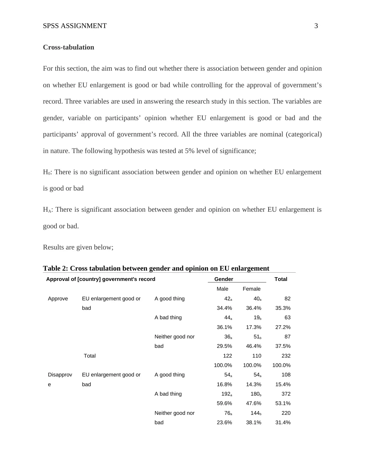
Table 2: Cross tabulation between gender and opinion on EU enlargement
Approval of [country] government's record Gender Total
Male Female
Approve EU enlargement good or
bad
A good thing 42a 40a 82
34.4% 36.4% 35.3%
A bad thing 44a 19b 63
36.1% 17.3% 27.2%
Neither good nor
bad
36a 51b 87
29.5% 46.4% 37.5%
Total 122 110 232
100.0% 100.0% 100.0%
Disapprov
e
EU enlargement good or
bad
A good thing 54a 54a 108
16.8% 14.3% 15.4%
A bad thing 192a 180b 372
59.6% 47.6% 53.1%
Neither good nor
bad
76a 144b 220
23.6% 38.1% 31.4%

SPSS ASSIGNMENT 4
Total 322 378 700
100.0% 100.0% 100.0%
Total EU enlargement good or
bad
A good thing 96a 94a 190
21.6% 19.3% 20.4%
A bad thing 236a 199b 435
53.2% 40.8% 46.7%
Neither good nor
bad
112a 195b 307
25.2% 40.0% 32.9%
Total 444 488 932
100.0% 100.0% 100.0%
Table 2: Chi-Square Tests
q86 approval of [country] government's record Value df Asymp. Sig.
(2-sided)
Approve Pearson Chi-Square 11.967b 2 .003
Likelihood Ratio 12.226 2 .002
Linear-by-Linear
Association
1.761 1 .185
N of Valid Cases 232
Disapprove Pearson Chi-Square 17.034c 2 .000
Likelihood Ratio 17.269 2 .000
Linear-by-Linear
Association
11.298 1 .001
N of Valid Cases 700
Total Pearson Chi-Square 23.583a 2 .000
Likelihood Ratio 23.815 2 .000
Linear-by-Linear
Association
13.111 1 .000
N of Valid Cases 932
a. 0 cells (0.0%) have expected count less than 5. The minimum expected count is 90.52.
b. 0 cells (0.0%) have expected count less than 5. The minimum expected count is 29.87.
c. 0 cells (0.0%) have expected count less than 5. The minimum expected count is 49.68.
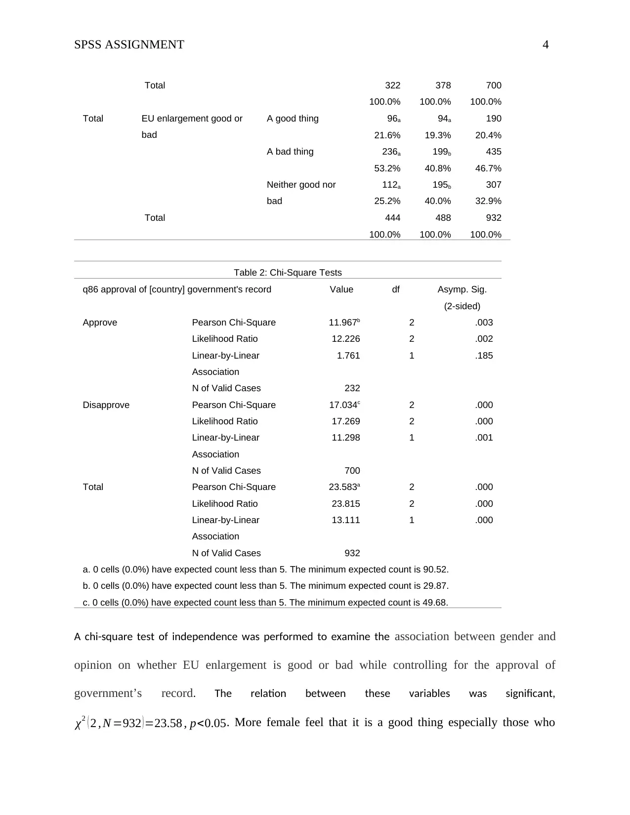
A chi-square test of independence was performed to examine the association between gender and
opinion on whether EU enlargement is good or bad while controlling for the approval of
government’s record. The relation between these variables was significant,
χ2 ( 2 , N =932 ) =23.58 , p<0.05. More female feel that it is a good thing especially those who

SPSS ASSIGNMENT 5
approved the government records. However, more of the male participants who disapproved the
government’s records felt that it was a good thing.
T-test analysis
For this section, we sought to test whether there is significant differences in the average years
lived in their current place of residence by the males and females. This was also tested at 5%
level of significance.
The variables used are gender and years lived in current residency. Gender is a categorical
variable while years lived in the current residency is a numerical variable.
The hypothesis that was tested is given as follows;
H0: There is significant difference in the number of years lived by the males and females in their
current place of residence.
HA: There is no significant difference in the number of years lived by the males and females in
their current place of residence.
Table 4: Group Statistics
Gender N Mean Std. Deviation Std. Error
Mean
Years residency in current
community
Male 456 18.99 16.086 .753
Female 523 19.84 15.869 .694
Table 5: Independent Samples Test
Levene's Test for
Equality of
Variances
t-test for Equality of Means
F Sig. t df Sig.
(2-
tailed)
Mean
Differe
nce
Std.
Error
Differe
nce
95% Confidence
Interval of the
Difference
Lower Upper

SPSS ASSIGNMENT 6
Years residency
in current
community
Equal
variances
assumed
.051 .821 -.837 977 .403 -.856 1.023 -2.864 1.152
Equal
variances
not
assumed
-.836 955.
248
.403 -.856 1.024 -2.866 1.154
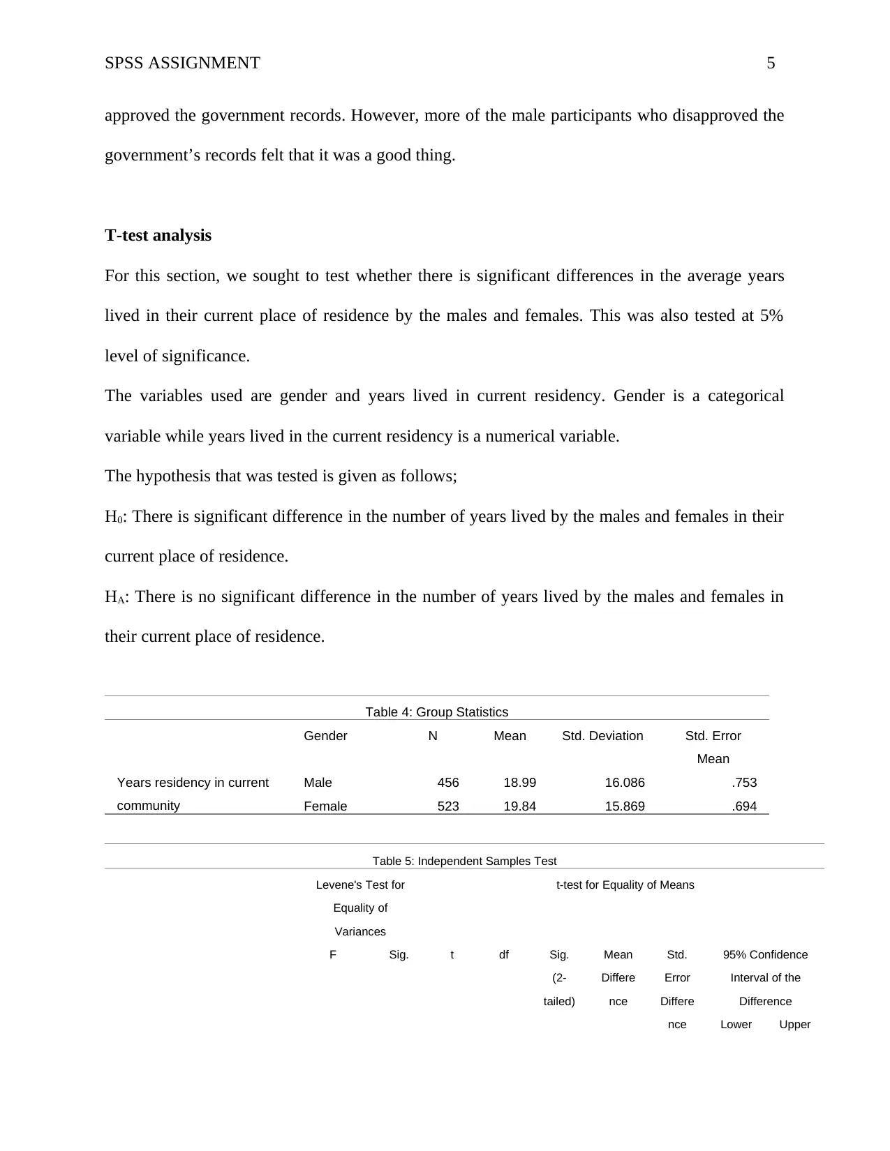
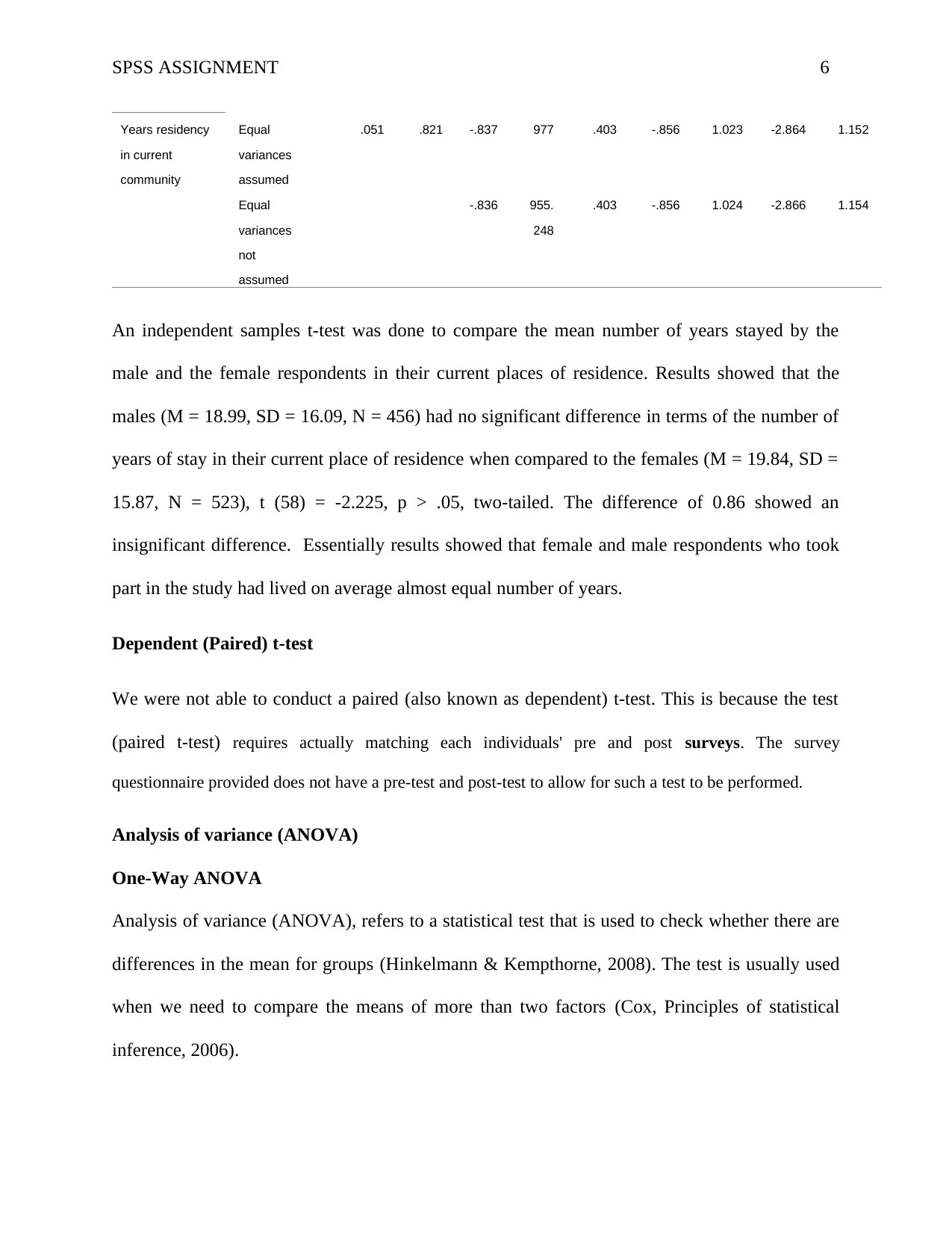
An independent samples t-test was done to compare the mean number of years stayed by the
male and the female respondents in their current places of residence. Results showed that the
males (M = 18.99, SD = 16.09, N = 456) had no significant difference in terms of the number of
years of stay in their current place of residence when compared to the females (M = 19.84, SD =
15.87, N = 523), t (58) = -2.225, p > .05, two-tailed. The difference of 0.86 showed an
insignificant difference. Essentially results showed that female and male respondents who took
part in the study had lived on average almost equal number of years.
Dependent (Paired) t-test
We were not able to conduct a paired (also known as dependent) t-test. This is because the test
(paired t-test) requires actually matching each individuals' pre and post surveys. The survey
questionnaire provided does not have a pre-test and post-test to allow for such a test to be performed.
Analysis of variance (ANOVA)
One-Way ANOVA
Analysis of variance (ANOVA), refers to a statistical test that is used to check whether there are
differences in the mean for groups (Hinkelmann & Kempthorne, 2008). The test is usually used
when we need to compare the means of more than two factors (Cox, Principles of statistical
inference, 2006).

SPSS ASSIGNMENT 7
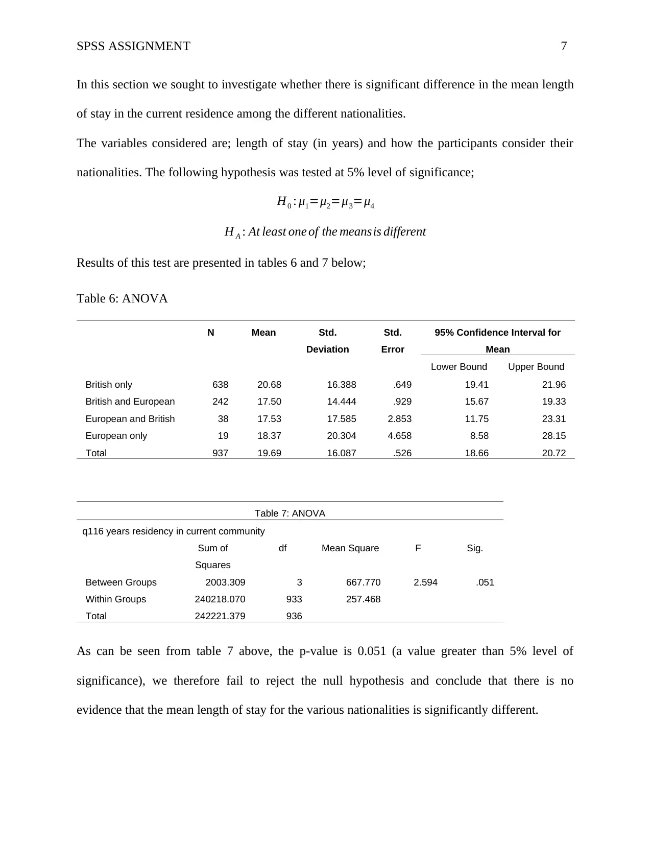
In this section we sought to investigate whether there is significant difference in the mean length
of stay in the current residence among the different nationalities.
The variables considered are; length of stay (in years) and how the participants consider their
nationalities. The following hypothesis was tested at 5% level of significance;
H0 : μ1=μ2=μ3=μ4
H A : At least one of the meansis different
Results of this test are presented in tables 6 and 7 below;
Table 6: ANOVA
N Mean Std.
Deviation
Std.
Error
95% Confidence Interval for
Mean
Lower Bound Upper Bound
British only 638 20.68 16.388 .649 19.41 21.96
British and European 242 17.50 14.444 .929 15.67 19.33
European and British 38 17.53 17.585 2.853 11.75 23.31
European only 19 18.37 20.304 4.658 8.58 28.15
Total 937 19.69 16.087 .526 18.66 20.72
Table 7: ANOVA
q116 years residency in current community
Sum of
Squares
df Mean Square F Sig.
Between Groups 2003.309 3 667.770 2.594 .051
Within Groups 240218.070 933 257.468
Total 242221.379 936
As can be seen from table 7 above, the p-value is 0.051 (a value greater than 5% level of
significance), we therefore fail to reject the null hypothesis and conclude that there is no
evidence that the mean length of stay for the various nationalities is significantly different.

SPSS ASSIGNMENT 8
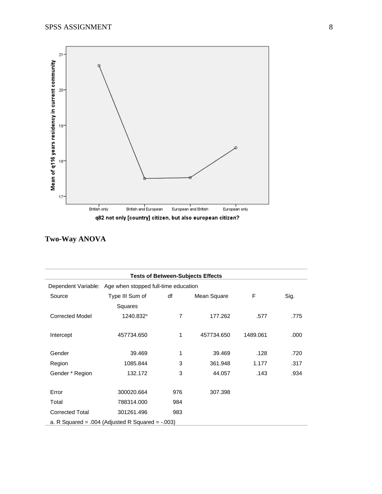
Two-Way ANOVA
Tests of Between-Subjects Effects
Dependent Variable: Age when stopped full-time education
Source Type III Sum of
Squares
df Mean Square F Sig.
Corrected Model 1240.832a 7 177.262 .577 .775
Intercept 457734.650 1 457734.650 1489.061 .000
Gender 39.469 1 39.469 .128 .720
Region 1085.844 3 361.948 1.177 .317
Gender * Region 132.172 3 44.057 .143 .934
Error 300020.664 976 307.398
Total 788314.000 984
Corrected Total 301261.496 983
a. R Squared = .004 (Adjusted R Squared = -.003)

SPSS ASSIGNMENT 9
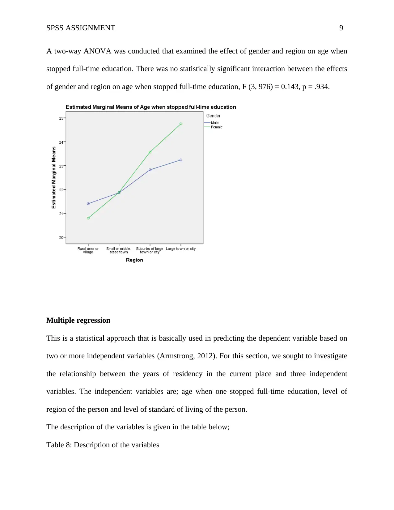
A two-way ANOVA was conducted that examined the effect of gender and region on age when
stopped full-time education. There was no statistically significant interaction between the effects
of gender and region on age when stopped full-time education, F (3, 976) = 0.143, p = .934.
Multiple regression
This is a statistical approach that is basically used in predicting the dependent variable based on
two or more independent variables (Armstrong, 2012). For this section, we sought to investigate
the relationship between the years of residency in the current place and three independent
variables. The independent variables are; age when one stopped full-time education, level of
region of the person and level of standard of living of the person.
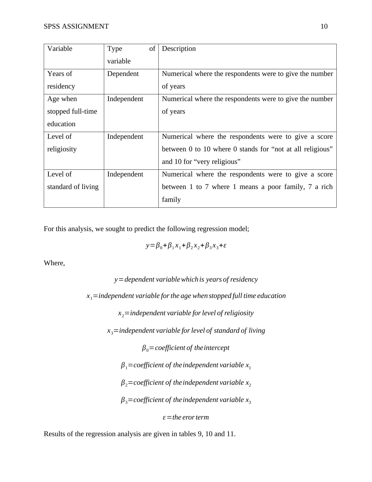
The description of the variables is given in the table below;
Table 8: Description of the variables

SPSS ASSIGNMENT 10
Variable Type of
variable
Description
Years of
residency
Dependent Numerical where the respondents were to give the number
of years
Age when
stopped full-time
education
Independent Numerical where the respondents were to give the number
of years
Level of
religiosity
Independent Numerical where the respondents were to give a score
between 0 to 10 where 0 stands for “not at all religious”
and 10 for “very religious”
Level of
standard of living
Independent Numerical where the respondents were to give a score
between 1 to 7 where 1 means a poor family, 7 a rich
family
For this analysis, we sought to predict the following regression model;
y=β0 + β1 x1 +β2 x2 + β3 x3 +ε
Where,
y=dependent variable which is years of residency
x1=independent variable for the age when stopped full time education
x2=independent variable for level of religiosity
x3=independent variable for level of standard of living
β0=coefficient of theintercept
β1=coefficient of theindependent variable x1
β2=coefficient of theindependent variable x2
β3=coefficient of theindependent variable x3
ε =the eror term
Results of the regression analysis are given in tables 9, 10 and 11.

SPSS ASSIGNMENT 11
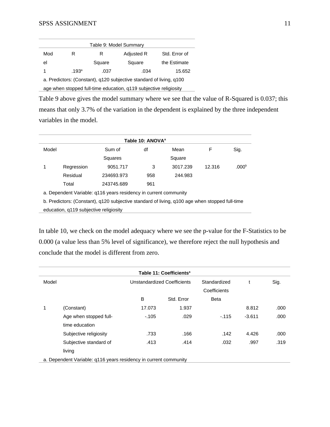
Table 9: Model Summary
Mod
el
R R
Square
Adjusted R
Square
Std. Error of
the Estimate
1 .193a .037 .034 15.652
a. Predictors: (Constant), q120 subjective standard of living, q100
age when stopped full-time education, q119 subjective religiosity
Table 9 above gives the model summary where we see that the value of R-Squared is 0.037; this
means that only 3.7% of the variation in the dependent is explained by the three independent
variables in the model.
Table 10: ANOVAa
Model Sum of
Squares
df Mean
Square
F Sig.
1 Regression 9051.717 3 3017.239 12.316 .000b
Residual 234693.973 958 244.983
Total 243745.689 961
a. Dependent Variable: q116 years residency in current community
b. Predictors: (Constant), q120 subjective standard of living, q100 age when stopped full-time
education, q119 subjective religiosity
In table 10, we check on the model adequacy where we see the p-value for the F-Statistics to be
0.000 (a value less than 5% level of significance), we therefore reject the null hypothesis and
conclude that the model is different from zero.
Table 11: Coefficientsa
Model Unstandardized Coefficients Standardized
Coefficients
t Sig.
B Std. Error Beta
1 (Constant) 17.073 1.937 8.812 .000
Age when stopped full-
time education
-.105 .029 -.115 -3.611 .000
Subjective religiosity .733 .166 .142 4.426 .000
Subjective standard of
living
.413 .414 .032 .997 .319
a. Dependent Variable: q116 years residency in current community

SPSS ASSIGNMENT 12
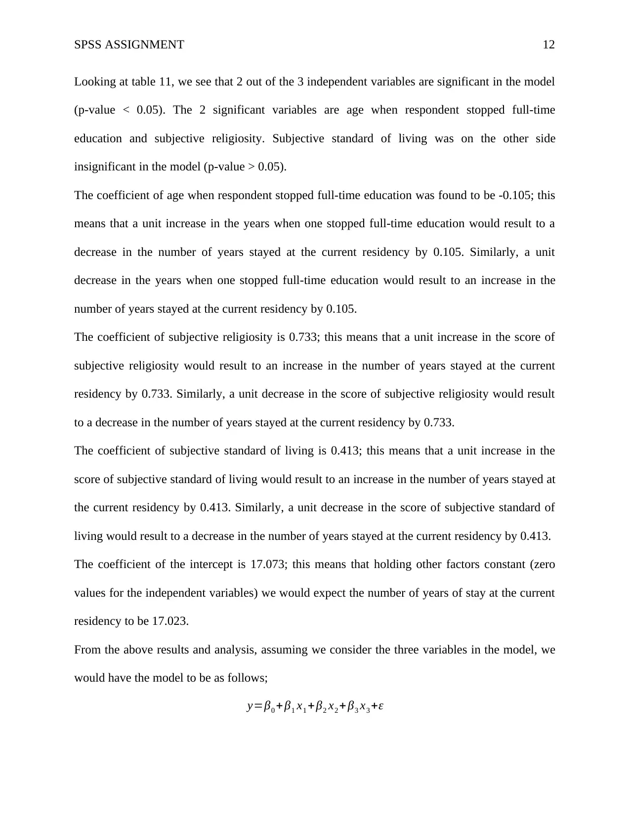
Looking at table 11, we see that 2 out of the 3 independent variables are significant in the model
(p-value < 0.05). The 2 significant variables are age when respondent stopped full-time
education and subjective religiosity. Subjective standard of living was on the other side
insignificant in the model (p-value > 0.05).
The coefficient of age when respondent stopped full-time education was found to be -0.105; this
means that a unit increase in the years when one stopped full-time education would result to a
decrease in the number of years stayed at the current residency by 0.105. Similarly, a unit
decrease in the years when one stopped full-time education would result to an increase in the
number of years stayed at the current residency by 0.105.
The coefficient of subjective religiosity is 0.733; this means that a unit increase in the score of
subjective religiosity would result to an increase in the number of years stayed at the current
residency by 0.733. Similarly, a unit decrease in the score of subjective religiosity would result
to a decrease in the number of years stayed at the current residency by 0.733.
The coefficient of subjective standard of living is 0.413; this means that a unit increase in the
score of subjective standard of living would result to an increase in the number of years stayed at
the current residency by 0.413. Similarly, a unit decrease in the score of subjective standard of
living would result to a decrease in the number of years stayed at the current residency by 0.413.
The coefficient of the intercept is 17.073; this means that holding other factors constant (zero
values for the independent variables) we would expect the number of years of stay at the current
residency to be 17.023.
From the above results and analysis, assuming we consider the three variables in the model, we
would have the model to be as follows;
y=β0 + β1 x1 +β2 x2 + β3 x3 +ε