SPSS: Hypothesis Testing, Regression, and Chi-Square Analysis

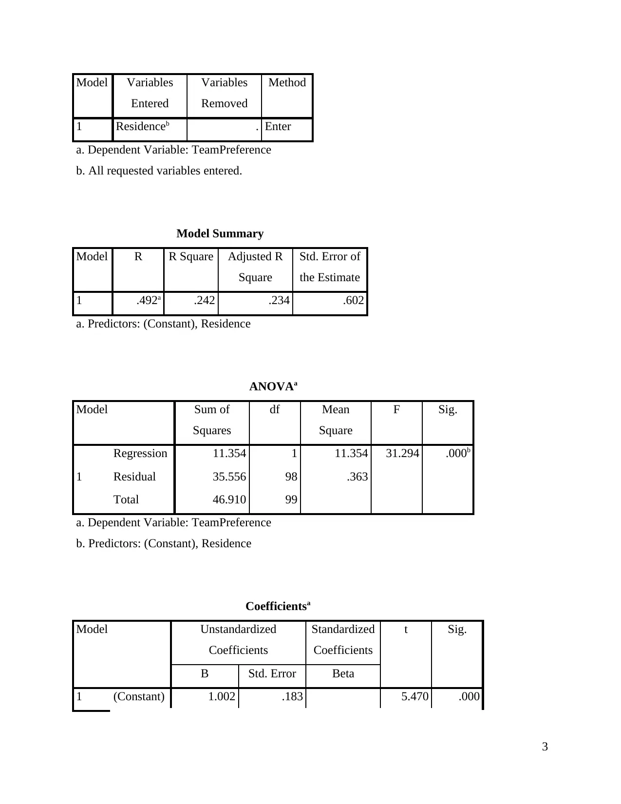
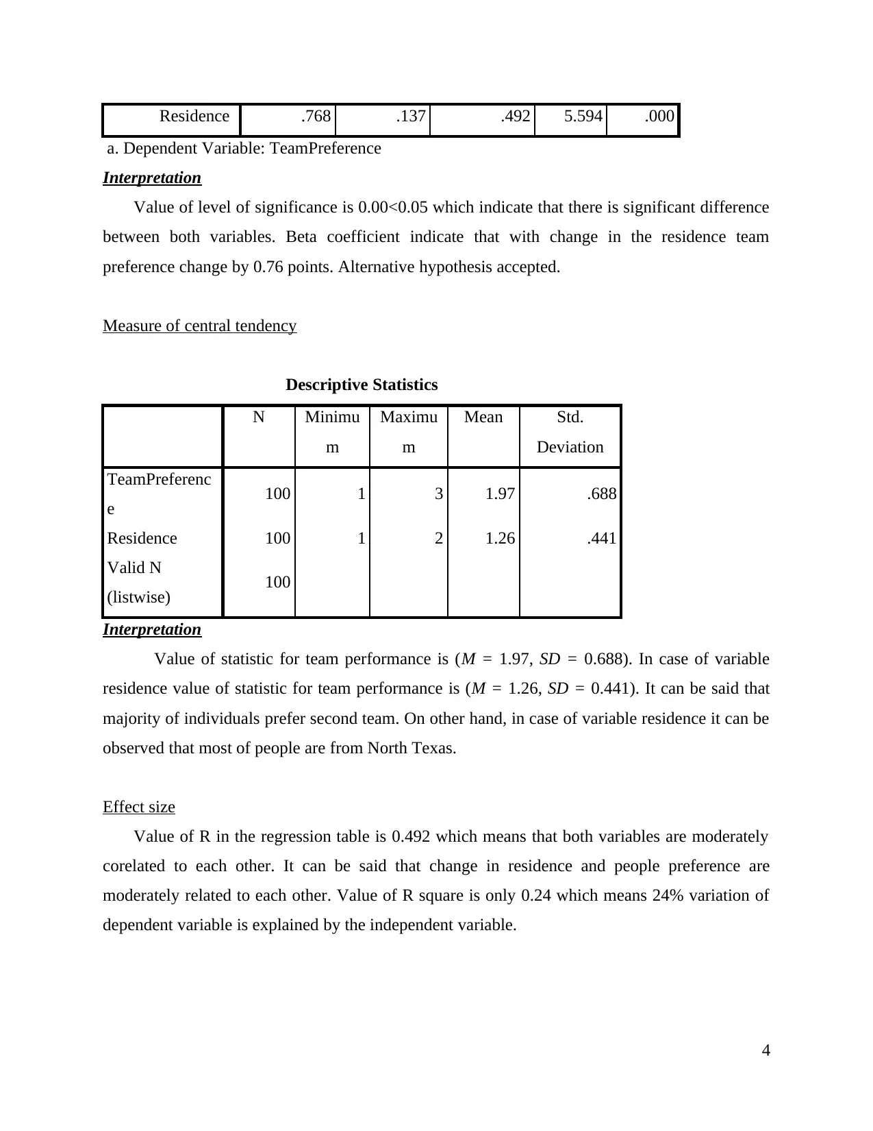
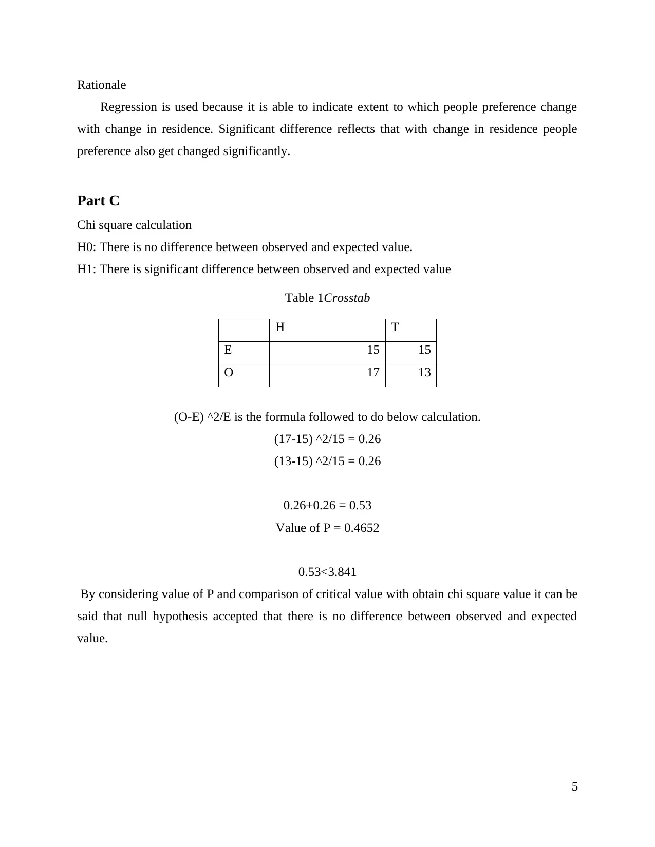
This SPSS assignment presents a statistical analysis of data, encompassing hypothesis testing, regression analysis, and chi-square calculations. Part A focuses on a one-sample t-test, stating null and research hypotheses, determining the measure of central tendency, calculating effect size, and ...Read More

SPSS

TABLE OF CONTENTS
Part A...............................................................................................................................................1
State your null & research hypotheses........................................................................................1
State the appropriate measure of central tendency for each variable..........................................2
Effect size....................................................................................................................................2
Rationale of choice of approach..................................................................................................2
Part B...............................................................................................................................................2
Regression analysis.....................................................................................................................2
Measure of central tendency.......................................................................................................4
Effect size....................................................................................................................................4
Rationale.....................................................................................................................................5
Part C...............................................................................................................................................5
Chi square calculation.................................................................................................................5

Part A
State your null & research hypotheses
H0: There is no significant difference between population mean and sample mean.
H1: There is significant difference between population mean and sample mean.
One-Sample Statistics
N Mean Std.
Deviation
Std. Error
Mean
TeamPreferenc
e 100 1.97 .688 .069
One-Sample Test
Test Value = 2
t df Sig. (2-
tailed)
Mean
Difference
95% Confidence Interval of
the Difference
Lower Upper
TeamPreferenc
e -.436 99 .664 -.030 -.17 .11
Interpretation
One sample t test indicate relationship between sample mean and population mean and
indicate whether there is significant difference between sample mean and population mean. In
the table given above it can be seen that value of statistics is (M = 1.97, SD = 0.688). This means
that on an average sample unit prefer Dallas Mavericks and standard deviation is very low which
further indicate that majority of respondents prefer mentioned team. Value of level of
significance is 0.069>0.05 which reflect that there is no significant mean difference between
sample mean and population mean. Null hypothesis accepted.
1

State the appropriate measure of central tendency for each variable
Descriptive Statistics
N Minimu
m
Maximu
m
Mean Std.
Deviation
TeamPreferenc
e 100 1 3 1.97 .688
Valid N
(listwise) 100
Value of statistics is (M = 1.97, SD = 0.688) and this indicate that average sample unit
prefer Dallas Mavericks.
Effect size
Mean difference -0.03
STDEV 5
Cohen d -0.006
Effect size is -0.006 which means that sample mean is -0.006 STDEV different from
population mean. Population mean and sample mean are closely related to each other.
Rationale of choice of approach
There is single variable and due to this reason one sample T test is used so as to find out
extent to which its mean is different from population mean. By doing so it is identified whether
sample is showing real picture relative to whatever really exists.
Part B
Regression analysis
H0: There is no significant impact of residence of people on their choice about team.
H1: There is significant impact of residence of people on their choice about team.
Variables Entered/Removeda
2

Model Variables
Entered
Variables
Removed
Method
1 Residenceb . Enter
a. Dependent Variable: TeamPreference
b. All requested variables entered.
Model Summary
Model R R Square Adjusted R
Square
Std. Error of
the Estimate
1 .492a .242 .234 .602
a. Predictors: (Constant), Residence
ANOVAa
Model Sum of
Squares
df Mean
Square
F Sig.
1
Regression 11.354 1 11.354 31.294 .000b
Residual 35.556 98 .363
Total 46.910 99
a. Dependent Variable: TeamPreference
b. Predictors: (Constant), Residence
Coefficientsa
Model Unstandardized
Coefficients
Standardized
Coefficients
t Sig.
B Std. Error Beta
1 (Constant) 1.002 .183 5.470 .000
3

Residence .768 .137 .492 5.594 .000
a. Dependent Variable: TeamPreference
Interpretation
Value of level of significance is 0.00<0.05 which indicate that there is significant difference
between both variables. Beta coefficient indicate that with change in the residence team
preference change by 0.76 points. Alternative hypothesis accepted.
Measure of central tendency
Descriptive Statistics
N Minimu
m
Maximu
m
Mean Std.
Deviation
TeamPreferenc
e 100 1 3 1.97 .688
Residence 100 1 2 1.26 .441
Valid N
(listwise) 100
Interpretation
Value of statistic for team performance is (M = 1.97, SD = 0.688). In case of variable
residence value of statistic for team performance is (M = 1.26, SD = 0.441). It can be said that
majority of individuals prefer second team. On other hand, in case of variable residence it can be
observed that most of people are from North Texas.
Effect size
Value of R in the regression table is 0.492 which means that both variables are moderately
corelated to each other. It can be said that change in residence and people preference are
moderately related to each other. Value of R square is only 0.24 which means 24% variation of
dependent variable is explained by the independent variable.
4

Rationale
Regression is used because it is able to indicate extent to which people preference change
with change in residence. Significant difference reflects that with change in residence people
preference also get changed significantly.
Part C
Chi square calculation
H0: There is no difference between observed and expected value.
H1: There is significant difference between observed and expected value
Table 1Crosstab
H T
E 15 15
O 17 13
(O-E) ^2/E is the formula followed to do below calculation.
(17-15) ^2/15 = 0.26
(13-15) ^2/15 = 0.26
0.26+0.26 = 0.53
Value of P = 0.4652
0.53<3.841
By considering value of P and comparison of critical value with obtain chi square value it can be
said that null hypothesis accepted that there is no difference between observed and expected
value.
5