SPSS Case Study: Examining Pain, Socioeconomic Groups, and MI

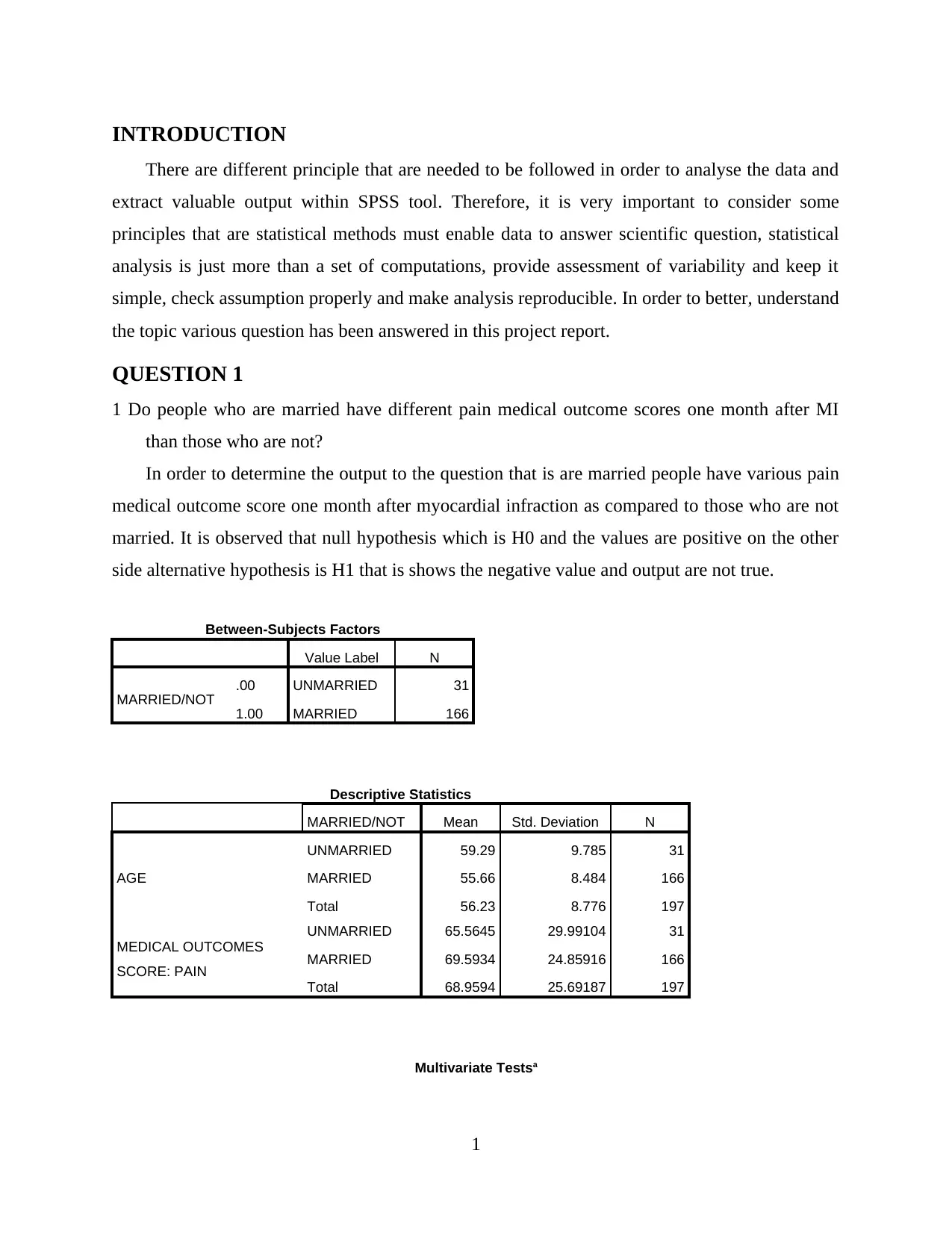
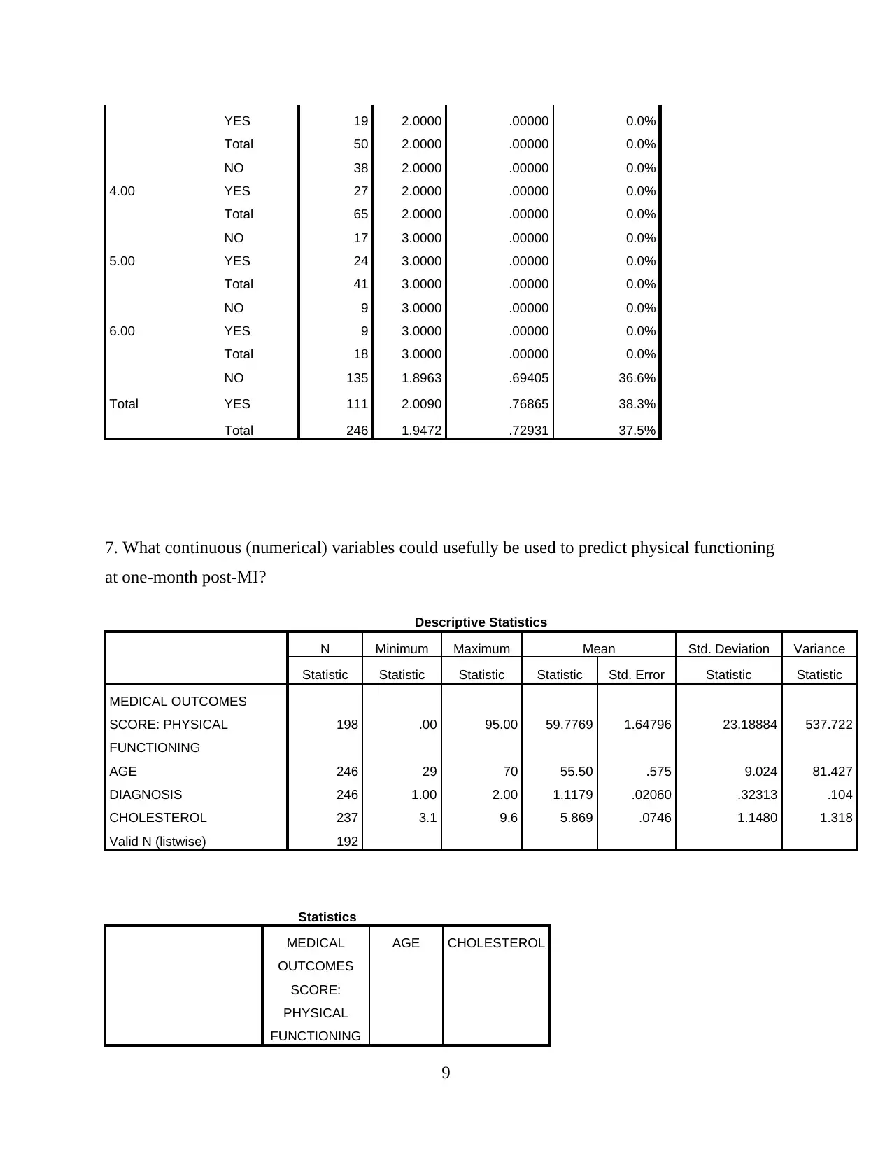
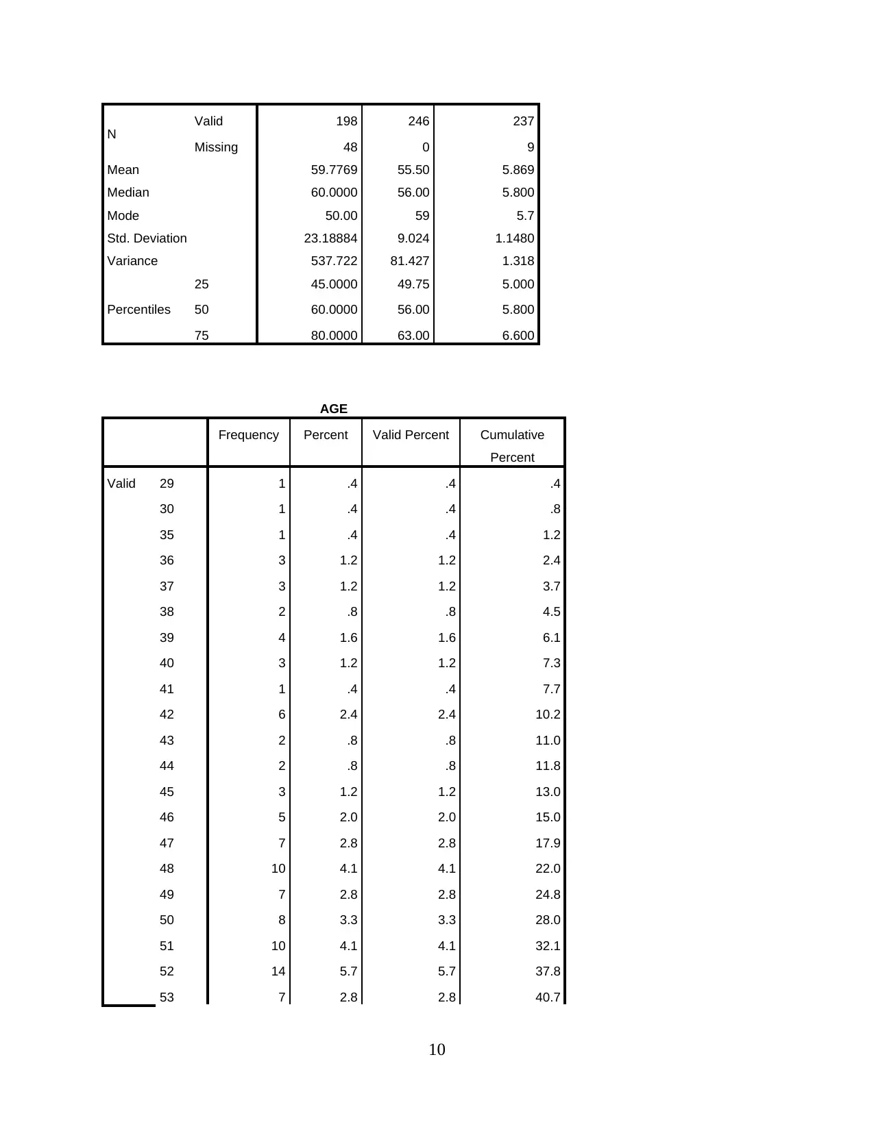
This SPSS case study examines medical data related to myocardial infarction (MI), pain outcomes, and socioeconomic factors. The analysis investigates whether marital status influences pain scores one month after MI, utilizing descriptive statistics, multivariate tests, and tests of between-subjects effects to compare groups. The study also explores the relationship between socioeconomic groups and pet ownership, employing one-sample tests and frequency distributions. Data includes variables such as age, medical outcomes scores, and social class. The findings provide insights into the impact of these factors on patient outcomes. The study uses various statistical methods to assess variability, check assumptions, and ensure reproducible analysis. The results are presented with statistical tables and figures to support the conclusions.

Case Study SPSS

INTRODUCTION
There are different principle that are needed to be followed in order to analyse the data and
extract valuable output within SPSS tool. Therefore, it is very important to consider some
principles that are statistical methods must enable data to answer scientific question, statistical
analysis is just more than a set of computations, provide assessment of variability and keep it
simple, check assumption properly and make analysis reproducible. In order to better, understand
the topic various question has been answered in this project report.
QUESTION 1
1 Do people who are married have different pain medical outcome scores one month after MI
than those who are not?
In order to determine the output to the question that is are married people have various pain
medical outcome score one month after myocardial infraction as compared to those who are not
married. It is observed that null hypothesis which is H0 and the values are positive on the other
side alternative hypothesis is H1 that is shows the negative value and output are not true.
Between-Subjects Factors
Value Label N
MARRIED/NOT .00 UNMARRIED 31
1.00 MARRIED 166
Descriptive Statistics
MARRIED/NOT Mean Std. Deviation N
AGE
UNMARRIED 59.29 9.785 31
MARRIED 55.66 8.484 166
Total 56.23 8.776 197
MEDICAL OUTCOMES
SCORE: PAIN
UNMARRIED 65.5645 29.99104 31
MARRIED 69.5934 24.85916 166
Total 68.9594 25.69187 197
Multivariate Testsa
1

Effect Value F Hypothesis
df
Error df Sig. Partial Eta
Squared
Noncent.
Parameter
Observed
Powerc
Intercept
Pillai's Trace .961 2403.659b 2.000 194.000 .000 .961 4807.318 1.000
Wilks'
Lambda .039 2403.659b 2.000 194.000 .000 .961 4807.318 1.000
Hotelling's
Trace 24.780 2403.659b 2.000 194.000 .000 .961 4807.318 1.000
Roy's
Largest Root 24.780 2403.659b 2.000 194.000 .000 .961 4807.318 1.000
marital
Pillai's Trace .029 2.929b 2.000 194.000 .056 .029 5.857 .566
Wilks'
Lambda .971 2.929b 2.000 194.000 .056 .029 5.857 .566
Hotelling's
Trace .030 2.929b 2.000 194.000 .056 .029 5.857 .566
Roy's
Largest Root .030 2.929b 2.000 194.000 .056 .029 5.857 .566
a. Design: Intercept + marital
b. Exact statistic
c. Computed using alpha = .05
MARRIED/NOT
Dependent Variable MARRIED/NOT Mean Std. Error 95% Confidence Interval
Lower Bound Upper Bound
AGE UNMARRIED 59.290 1.562 56.210 62.371
MARRIED 55.657 .675 54.325 56.988
MEDICAL OUTCOMES
SCORE: PAIN
UNMARRIED 65.565 4.619 56.456 74.673
MARRIED 69.593 1.996 65.657 73.530
2

The above answer are extracted with the use of multivariate test and descriptive analysis
because it help to figure out the exact values of married people that have different pain outcome
score with relation to MI. This statistical analysis provides the meaningful result like mean,
standard deviation between total age of married and unmarried and the medical outcomes score
pain with both dependent variable. From the SPSS result, it has been observed that yes married
people have more and assorted pain medical score as compared to unmarried.
QUSETION 2:
2. Is there a difference in depression level following MI between those who have pets and those
who do not?
The following result are demonstrated with the support of chi square test as it will deliver
better result as compared to any other method. This is a procedure for an independence test that
produces the two categorical variable that are related to the same class interval.
Case Processing Summary
Cases
Valid Missing Total
N Percent N Percent N Percent
DEPRESSION * PETS 197 80.1% 49 19.9% 246 100.0%
3

Chi-Square Tests
Value df Asymp. Sig. (2-
sided)
Pearson Chi-Square 195.229a 172 .108
Likelihood Ratio 151.383 172 .869
Linear-by-Linear Association .074 1 .786
N of Valid Cases 197
a. 216 cells (98.2%) have expected count less than 5. The minimum
expected count is .02.
Statistics
DEPRESSION PETS Y/N
N Valid 197 246
Missing 49 0
Mean 13.6751 .4512
Median 11.0000 .0000
Mode 1.00 .00
Std. Deviation 11.79960 .49863
DEPRESSION
Frequency Percent Valid Percent Cumulative
Percent
Valid .00 9 3.7 4.6 4.6
1.00 14 5.7 7.1 11.7
2.00 9 3.7 4.6 16.2
3.00 11 4.5 5.6 21.8
4.00 13 5.3 6.6 28.4
5.00 9 3.7 4.6 33.0
6.00 5 2.0 2.5 35.5
7.00 8 3.3 4.1 39.6
8.00 6 2.4 3.0 42.6
9.00 11 4.5 5.6 48.2
10.00 3 1.2 1.5 49.7
11.00 9 3.7 4.6 54.3
12.00 3 1.2 1.5 55.8
13.00 1 .4 .5 56.3
4

14.00 3 1.2 1.5 57.9
15.00 3 1.2 1.5 59.4
16.00 6 2.4 3.0 62.4
17.00 8 3.3 4.1 66.5
18.00 5 2.0 2.5 69.0
19.00 8 3.3 4.1 73.1
20.00 6 2.4 3.0 76.1
21.00 1 .4 .5 76.6
22.00 4 1.6 2.0 78.7
23.00 6 2.4 3.0 81.7
24.00 3 1.2 1.5 83.2
25.00 3 1.2 1.5 84.8
26.00 2 .8 1.0 85.8
27.00 3 1.2 1.5 87.3
28.00 4 1.6 2.0 89.3
29.00 1 .4 .5 89.8
30.00 4 1.6 2.0 91.9
31.00 1 .4 .5 92.4
32.00 1 .4 .5 92.9
34.00 2 .8 1.0 93.9
35.00 1 .4 .5 94.4
37.00 1 .4 .5 94.9
38.00 2 .8 1.0 95.9
40.00 2 .8 1.0 97.0
44.00 1 .4 .5 97.5
45.00 1 .4 .5 98.0
46.00 1 .4 .5 98.5
49.00 1 .4 .5 99.0
51.00 1 .4 .5 99.5
58.00 1 .4 .5 100.0
Total 197 80.1 100.0
Missing System 49 19.9
Total 246 100.0
PETS Y/N
5

Frequency Percent Valid Percent Cumulative
Percent
Valid
NO 135 54.9 54.9 54.9
YES 111 45.1 45.1 100.0
Total 246 100.0 100.0
5. Do people with differing cardiac diagnoses have different levels of mental health outcomes at
one-month post-MI?
There is a systematic approach to determine the values of different level of mental health
outcome at one-month post myocardial infraction that one way ancova test. This is also consider
as univariate test that is the simplest form, for analysing the data that show the differences in one
variable. It determine the patter within available data and describe the univariate information
which includes mean, mode, median and useful dispersion. From the result it has been analysed
that total number of observation are 173 and mean of mental health with cardiac diagnosis is
60.232 and standard deviation is 22.78315 and the mean square from univariate test shows that
people with assorted diagnoses have different level of mental health outcome before MI.
Between-Subjects Factors
Value Label N
DIAGNOSIS 1.00 MI 173
Descriptive Statistics
Dependent Variable: MEDICAL OUTCOMES SCORE:
PHYSICAL FUNCTIONING
DIAGNOSIS Mean Std. Deviation N
MI 60.2232 22.78315 173
Total 60.2232 22.78315 173
Tests of Between-Subjects Effects
Dependent Variable: MEDICAL OUTCOMES SCORE: PHYSICAL FUNCTIONING
Source Type III Sum of
Squares
df Mean Square F Sig. Partial Eta
Squared
Corrected Model 539.197a 1 539.197 1.039 .309 .006
Intercept 321237.699 1 321237.699 619.010 .000 .784
mv09 539.197 1 539.197 1.039 .309 .006
mv08 .000 0 . . . .000
Error 88741.151 171 518.954
6

Total 716722.299 173
Corrected Total 89280.349 172
a. R Squared = .006 (Adjusted R Squared = .000)
Estimates
Dependent Variable: MEDICAL OUTCOMES SCORE: PHYSICAL
FUNCTIONING
DIAGNOSIS Mean Std. Error 95% Confidence Interval
Lower Bound Upper Bound
MI 60.223a 1.732 56.804 63.642
a. Covariates appearing in the model are evaluated at the following values:
SITE OF MI = 3.06.
Univariate Tests
Dependent Variable: MEDICAL OUTCOMES SCORE: PHYSICAL FUNCTIONING
Sum of Squares df Mean Square F Sig. Partial Eta
Squared
Contrast .000 0 . . . .000
Error 88741.151 171 518.954
The F tests the effect of DIAGNOSIS. This test is based on the linearly independent pairwise
comparisons among the estimated marginal means.
6. Is there a difference in the proportions of pet owners in upper, middle and lower socio-
economic groups?
It is very important to determine the differences in proportion of two variable that can be
complete with the support of one sample test and frequency distribution.
One-Sample Statistics
N Mean Std. Deviation Std. Error Mean
SOCIAL CLASS
CATEGORY (3) 246 1.9472 .72931 .04650
PETS Y/N 246 .4512 .49863 .03179
One-Sample Test
Test Value = 0
7

t df Sig. (2-tailed) Mean Difference 95% Confidence Interval of the
Difference
Lower Upper
SOCIAL CLASS CATEGORY
(3) 41.875 245 .000 1.94715 1.8556 2.0387
PETS Y/N 14.193 245 .000 .45122 .3886 .5138
Descriptive
SOCIAL CLASS CATEGORY (3)
N Mean Std. Deviation Std. Error 95% Confidence Interval for Mean Minimum Maximum
Lower Bound Upper Bound
NONE 135 1.8963 .69405 .05973 1.7782 2.0144 1.00 3.00
DOGS 68 1.9853 .81940 .09937 1.7870 2.1836 1.00 3.00
CATS 18 2.0556 .63914 .15065 1.7377 2.3734 1.00 3.00
OTHER 5 2.0000 .70711 .31623 1.1220 2.8780 1.00 3.00
MIXTURE 20 2.0500 .75915 .16975 1.6947 2.4053 1.00 3.00
Total 246 1.9472 .72931 .04650 1.8556 2.0387 1.00 3.00
ANOVA
SOCIAL CLASS CATEGORY (3)
Sum of Squares df Mean Square F Sig.
Between Groups .885 4 .221 .412 .800
Within Groups 129.428 241 .537
Total 130.313 245
Descriptive Statistics
SOCIAL CLASS CATEGORY (3)
SOCIAL CLASS PETS Y/N Count Mean Standard
Deviation
Coefficient of
Variation
1.00
NO 4 1.0000 .00000 0.0%
YES 8 1.0000 .00000 0.0%
Total 12 1.0000 .00000 0.0%
2.00
NO 36 1.0000 .00000 0.0%
YES 24 1.0000 .00000 0.0%
Total 60 1.0000 .00000 0.0%
3.00 NO 31 2.0000 .00000 0.0%
8

YES 19 2.0000 .00000 0.0%
Total 50 2.0000 .00000 0.0%
4.00
NO 38 2.0000 .00000 0.0%
YES 27 2.0000 .00000 0.0%
Total 65 2.0000 .00000 0.0%
5.00
NO 17 3.0000 .00000 0.0%
YES 24 3.0000 .00000 0.0%
Total 41 3.0000 .00000 0.0%
6.00
NO 9 3.0000 .00000 0.0%
YES 9 3.0000 .00000 0.0%
Total 18 3.0000 .00000 0.0%
Total
NO 135 1.8963 .69405 36.6%
YES 111 2.0090 .76865 38.3%
Total 246 1.9472 .72931 37.5%
7. What continuous (numerical) variables could usefully be used to predict physical functioning
at one-month post-MI?
Descriptive Statistics
N Minimum Maximum Mean Std. Deviation Variance
Statistic Statistic Statistic Statistic Std. Error Statistic Statistic
MEDICAL OUTCOMES
SCORE: PHYSICAL
FUNCTIONING
198 .00 95.00 59.7769 1.64796 23.18884 537.722
AGE 246 29 70 55.50 .575 9.024 81.427
DIAGNOSIS 246 1.00 2.00 1.1179 .02060 .32313 .104
CHOLESTEROL 237 3.1 9.6 5.869 .0746 1.1480 1.318
Valid N (listwise) 192
Statistics
MEDICAL
OUTCOMES
SCORE:
PHYSICAL
FUNCTIONING
AGE CHOLESTEROL
9

N Valid 198 246 237
Missing 48 0 9
Mean 59.7769 55.50 5.869
Median 60.0000 56.00 5.800
Mode 50.00 59 5.7
Std. Deviation 23.18884 9.024 1.1480
Variance 537.722 81.427 1.318
Percentiles
25 45.0000 49.75 5.000
50 60.0000 56.00 5.800
75 80.0000 63.00 6.600
AGE
Frequency Percent Valid Percent Cumulative
Percent
Valid 29 1 .4 .4 .4
30 1 .4 .4 .8
35 1 .4 .4 1.2
36 3 1.2 1.2 2.4
37 3 1.2 1.2 3.7
38 2 .8 .8 4.5
39 4 1.6 1.6 6.1
40 3 1.2 1.2 7.3
41 1 .4 .4 7.7
42 6 2.4 2.4 10.2
43 2 .8 .8 11.0
44 2 .8 .8 11.8
45 3 1.2 1.2 13.0
46 5 2.0 2.0 15.0
47 7 2.8 2.8 17.9
48 10 4.1 4.1 22.0
49 7 2.8 2.8 24.8
50 8 3.3 3.3 28.0
51 10 4.1 4.1 32.1
52 14 5.7 5.7 37.8
53 7 2.8 2.8 40.7
10