SPSS Regression and Time Series Analysis

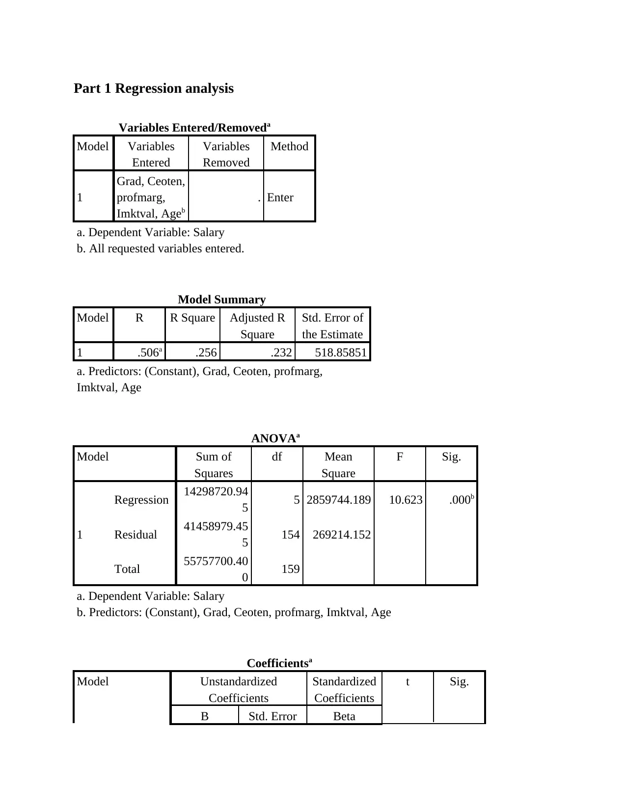
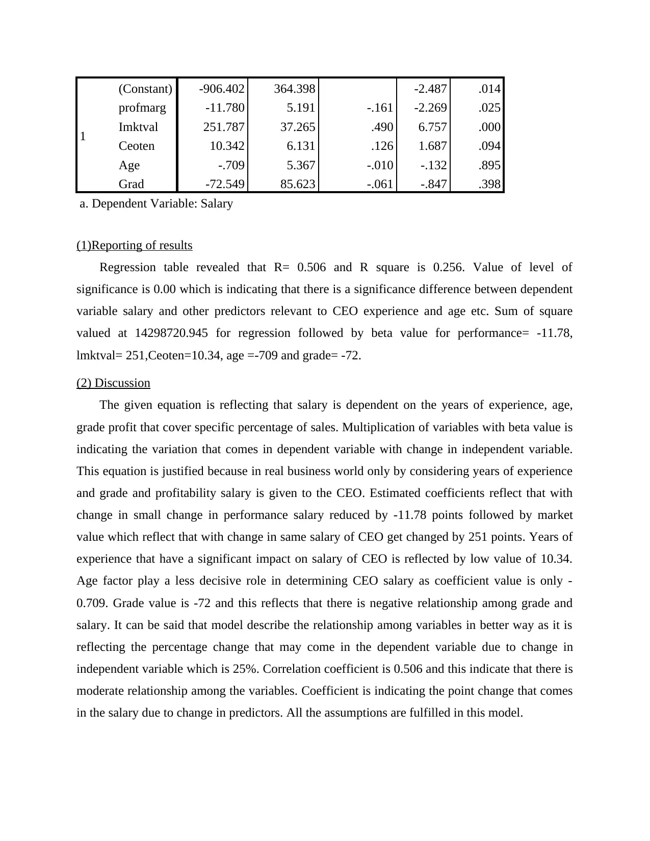
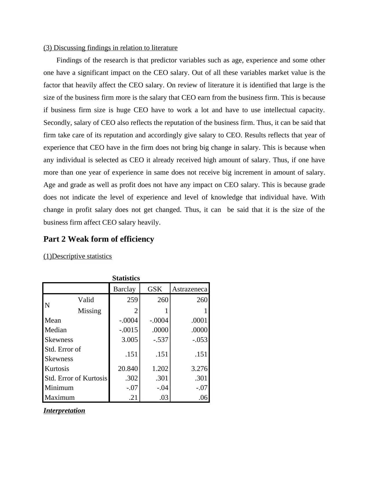
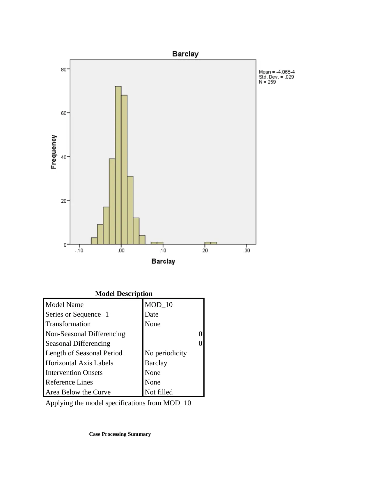
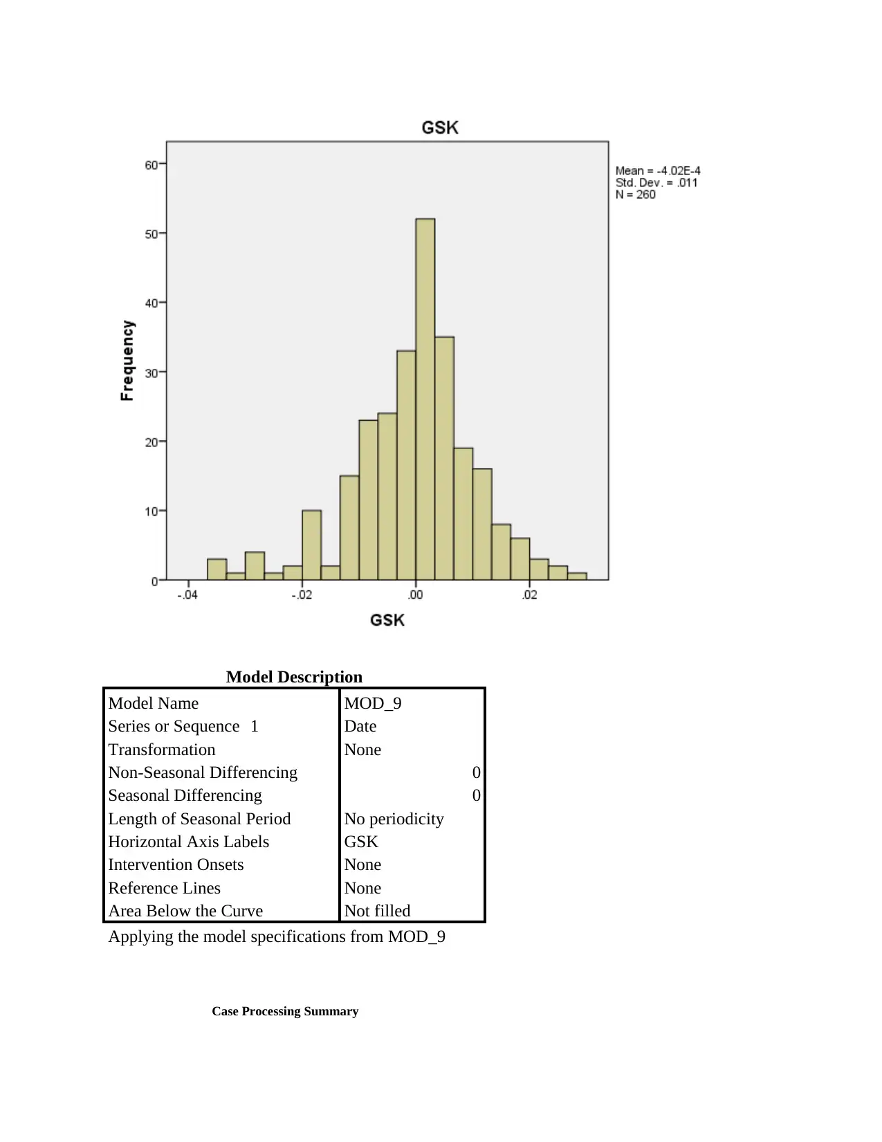
This report presents a comprehensive analysis of financial data using SPSS statistical software. The report is divided into two main parts. Part 1 focuses on regression analysis to determine the factors influencing CEO salaries. It details the regression model, reports the results (R, R-squared, ANOVA, coefficients), discusses the findings in relation to existing literature, and interprets the significance of variables like experience, age, and market value. Part 2 investigates the weak form of market efficiency by analyzing the daily returns of three companies (Barclay, GSK, and AstraZeneca). Descriptive statistics are presented, followed by an autoregressive model analysis for each company to assess the impact of lagged returns on current returns. The report also examines the day-of-the-week effect on returns. Overall, the report demonstrates the application of statistical methods to analyze financial data and draw meaningful conclusions about CEO compensation and market efficiency.

SPSS

TABLE OF CONTENTS
Part 1 Regression analysis...............................................................................................................3
(1)Reporting of results.................................................................................................................4
(2) Discussion..............................................................................................................................4
(3) Discussing findings in relation to literature...........................................................................5
Part 2 Weak form of efficiency.......................................................................................................5
(1)Descriptive statistics...............................................................................................................5
2 Autoregressive model.............................................................................................................12
3 Days of effect..............................................................................................................................16

Part 1 Regression analysis
Variables Entered/Removeda
Model Variables
Entered
Variables
Removed
Method
1
Grad, Ceoten,
profmarg,
Imktval, Ageb
. Enter
a. Dependent Variable: Salary
b. All requested variables entered.
Model Summary
Model R R Square Adjusted R
Square
Std. Error of
the Estimate
1 .506a .256 .232 518.85851
a. Predictors: (Constant), Grad, Ceoten, profmarg,
Imktval, Age
ANOVAa
Model Sum of
Squares
df Mean
Square
F Sig.
1
Regression 14298720.94
5 5 2859744.189 10.623 .000b
Residual 41458979.45
5 154 269214.152
Total 55757700.40
0 159
a. Dependent Variable: Salary
b. Predictors: (Constant), Grad, Ceoten, profmarg, Imktval, Age
Coefficientsa
Model Unstandardized
Coefficients
Standardized
Coefficients
t Sig.
B Std. Error Beta

1
(Constant) -906.402 364.398 -2.487 .014
profmarg -11.780 5.191 -.161 -2.269 .025
Imktval 251.787 37.265 .490 6.757 .000
Ceoten 10.342 6.131 .126 1.687 .094
Age -.709 5.367 -.010 -.132 .895
Grad -72.549 85.623 -.061 -.847 .398
a. Dependent Variable: Salary
(1)Reporting of results
Regression table revealed that R= 0.506 and R square is 0.256. Value of level of
significance is 0.00 which is indicating that there is a significance difference between dependent
variable salary and other predictors relevant to CEO experience and age etc. Sum of square
valued at 14298720.945 for regression followed by beta value for performance= -11.78,
lmktval= 251,Ceoten=10.34, age =-709 and grade= -72.
(2) Discussion
The given equation is reflecting that salary is dependent on the years of experience, age,
grade profit that cover specific percentage of sales. Multiplication of variables with beta value is
indicating the variation that comes in dependent variable with change in independent variable.
This equation is justified because in real business world only by considering years of experience
and grade and profitability salary is given to the CEO. Estimated coefficients reflect that with
change in small change in performance salary reduced by -11.78 points followed by market
value which reflect that with change in same salary of CEO get changed by 251 points. Years of
experience that have a significant impact on salary of CEO is reflected by low value of 10.34.
Age factor play a less decisive role in determining CEO salary as coefficient value is only -
0.709. Grade value is -72 and this reflects that there is negative relationship among grade and
salary. It can be said that model describe the relationship among variables in better way as it is
reflecting the percentage change that may come in the dependent variable due to change in
independent variable which is 25%. Correlation coefficient is 0.506 and this indicate that there is
moderate relationship among the variables. Coefficient is indicating the point change that comes
in the salary due to change in predictors. All the assumptions are fulfilled in this model.

(3) Discussing findings in relation to literature
Findings of the research is that predictor variables such as age, experience and some other
one have a significant impact on the CEO salary. Out of all these variables market value is the
factor that heavily affect the CEO salary. On review of literature it is identified that large is the
size of the business firm more is the salary that CEO earn from the business firm. This is because
if business firm size is huge CEO have to work a lot and have to use intellectual capacity.
Secondly, salary of CEO also reflects the reputation of the business firm. Thus, it can be said that
firm take care of its reputation and accordingly give salary to CEO. Results reflects that year of
experience that CEO have in the firm does not bring big change in salary. This is because when
any individual is selected as CEO it already received high amount of salary. Thus, if one have
more than one year of experience in same does not receive big increment in amount of salary.
Age and grade as well as profit does not have any impact on CEO salary. This is because grade
does not indicate the level of experience and level of knowledge that individual have. With
change in profit salary does not get changed. Thus, it can be said that it is the size of the
business firm affect CEO salary heavily.
Part 2 Weak form of efficiency
(1)Descriptive statistics
Statistics
Barclay GSK Astrazeneca
N Valid 259 260 260
Missing 2 1 1
Mean -.0004 -.0004 .0001
Median -.0015 .0000 .0000
Skewness 3.005 -.537 -.053
Std. Error of
Skewness .151 .151 .151
Kurtosis 20.840 1.202 3.276
Std. Error of Kurtosis .302 .301 .301
Minimum -.07 -.04 -.07
Maximum .21 .03 .06
Interpretation

Model Description
Model Name MOD_10
Series or Sequence 1 Date
Transformation None
Non-Seasonal Differencing 0
Seasonal Differencing 0
Length of Seasonal Period No periodicity
Horizontal Axis Labels Barclay
Intervention Onsets None
Reference Lines None
Area Below the Curve Not filled
Applying the model specifications from MOD_10
Case Processing Summary

Date
Series or Sequence Length 261
Number of Missing
Values in the Plot
User-Missing 0
System-
Missing 0

Model Description
Model Name MOD_9
Series or Sequence 1 Date
Transformation None
Non-Seasonal Differencing 0
Seasonal Differencing 0
Length of Seasonal Period No periodicity
Horizontal Axis Labels GSK
Intervention Onsets None
Reference Lines None
Area Below the Curve Not filled
Applying the model specifications from MOD_9
Case Processing Summary

Date
Series or Sequence Length 261
Number of Missing
Values in the Plot
User-Missing 0
System-
Missing 0

Model Description
Model Name MOD_8
Series or Sequence 1 Date
Transformation None
Non-Seasonal Differencing 0
Seasonal Differencing 0
Length of Seasonal Period No periodicity
Horizontal Axis Labels Astrazeneca
Intervention Onsets None
Reference Lines None
Area Below the Curve Not filled
Applying the model specifications from MOD_8
Case Processing Summary

Date
Series or Sequence Length 261
Number of Missing
Values in the Plot
User-Missing 0
System-
Missing 0
Results reflected that mean value of Barclay and GSK is -0.04 and this means on average
basis negative return is generated by the both firms. In case of AstraZeneca return percentage is
0.0001 which is also very low which reflects that all these three firms give very less percentage
of return to the investors. Median value is almost 0.000 which reflects that almost most of times
same return is given by the firms to the investors and due to this reason median value almost
stood at 0.000. Skewness value is 3.005 for Barclay -0.537 and for AstraZeneca same is -0.53

which reflects that data is not normally distributed because value of all variables is not equal to
1. Same things are reflected by Kurtosis. There is a huge difference between minimum and
maximum value of return for Barclay and AstraZeneca. Minimum and maximum value for
Barclay is -0.07 and 0.21 and this indicate that there is wide gap between positive and negative
return that is given to the investors. This gap is very low in case of GSK and AstraZeneca and on
this basis it can be said that both firms lagged behind Barclay in terms of performance.
2 Autoregressive model
GSK
Variables Entered/Removeda
Model Variables
Entered
Variables
Removed
Method
1 LAGGSKb . Enter
a. Dependent Variable: GSK
b. All requested variables entered.
Model Summary
Model R R Square Adjusted R
Square
Std. Error of
the Estimate
1 .718a .515 .513 .00746
a. Predictors: (Constant), LAGGSK
ANOVAa
Model Sum of
Squares
df Mean
Square
F Sig.
1 Regression .015 1 .015 274.330 .000b
Residual .014 258 .000

Total .030 259
a. Dependent Variable: GSK
b. Predictors: (Constant), LAGGSK
Coefficientsa
Model Unstandardized
Coefficients
Standardized
Coefficients
t Sig.
B Std. Error Beta
1 (Constant) -2.734E-007 .000 -.001 1.000
LAGGSK .499 .030 .718 16.563 .000
a. Dependent Variable: GSK
Interpretation
R square value is 51% and R valued at 0.71and this reflect that due to change in log
variable GSK share price will change by 51% in a day. Value of level of significance is 0.00 and
this indicate that there is significance difference between independent and dependent variable.
Coefficient is reflect that due to change in lag value change of 0.49 point comes in the firm share
price. It can be said that lag value significantly affect the share price of GSK.
AstraZeneca
Variables Entered/Removeda
Model Variables
Entered
Variables
Removed
Method
1 LAGASTRA
ZENECAb . Enter
a. Dependent Variable: Astrazeneca
b. All requested variables entered.

Model Summary
Model R R Square Adjusted R
Square
Std. Error of
the Estimate
1 .159a .025 .021 .01450
a. Predictors: (Constant), LAGASTRAZENECA
ANOVAa
Model Sum of
Squares
df Mean
Square
F Sig.
1
Regression .001 1 .001 6.687 .010b
Residual .054 258 .000
Total .056 259
a. Dependent Variable: Astrazeneca
b. Predictors: (Constant), LAGASTRAZENECA
Coefficientsa
Model Unstandardized
Coefficients
Standardized
Coefficients
t Sig.
B Std. Error Beta
1
(Constant) 4.552E-005 .001 .051 .960
LAGASTRAZEN
ECA .105 .041 .159 2.586 .010
a. Dependent Variable: Astrazeneca
Interpretation
Value of R and R square is 0.159 and 2% and this means that due to change in lag values
2% change will come in the share price of AstraZeneca. Level of significant difference is
observed 0.010>0.05 and this means that there is a significance difference in the returns that are
generated on daily basis by the AstraZeneca. Value of coefficient is 0.105 and this means that

with change in independent variable share price of the mentioned company changed by 0.105
points on daily basis. Thus, moderate return can be earned by the investors on investment.
Barclay
Variables Entered/Removeda
Model Variables
Entered
Variables
Removed
Method
1 LAGBARCL
AYb . Enter
a. Dependent Variable: Barclay
b. All requested variables entered.
Model Summary
Model R R Square Adjusted R
Square
Std. Error of
the Estimate
1 .037a .001 -.003 .02733
a. Predictors: (Constant), LAGBARCLAY
ANOVAa
Model Sum of
Squares
df Mean
Square
F Sig.
1
Regression .000 1 .000 .353 .553b
Residual .192 257 .001
Total .192 258
a. Dependent Variable: Barclay
b. Predictors: (Constant), LAGBARCLAY

Coefficientsa
Model Unstandardized
Coefficients
Standardized
Coefficients
t Sig.
B Std. Error Beta
1
(Constant) .001 .002 .660 .510
LAGBARCL
AY .025 .042 .037 .594 .553
a. Dependent Variable: Barclay
Interpretation
R and R square value is 0.37 and 0.01 and this means that there is low correlation among
the variables and due to change in one variable 0.01% change comes in other variable. Level of
significant difference is 0.553>0.05 and this reflects that big variation does not come in the
dependent variable due to change in independent variable. This is further validate from the fact
that value of coefficient is 0.025 which means that with change in independent variable only
variation of 0.025 comes in the dependent variable. Hence, one who is risk averse in nature can
make investment in Barclay.
3 Days of effect
Variables Entered/Removeda
Mode
l
Variables
Entered
Variables
Removed
Method
1 Mondayb . Enter
a. Dependent Variable: y
b. All requested variables entered.

Model Summary
Mode
l
R R
Square
Adjusted R
Square
Std. Error
of the
Estimate
1 .544a .296 .061 .00592
a. Predictors: (Constant), Monday
ANOVAa
Model Sum of
Squares
df Mean
Square
F Sig.
1
Regressio
n .000 1 .000 1.259 .344b
Residual .000 3 .000
Total .000 4
a. Dependent Variable: y
b. Predictors: (Constant), Monday
Coefficientsa
Model Unstandardized
Coefficients
Standardize
d
Coefficient
s
t Sig.
B Std. Error Beta