SPSS Report: Statistical Analysis and Hypothesis Testing Results
VerifiedAdded on 2021/02/18
|14
|2600
|94
Report
AI Summary
This SPSS report presents a detailed statistical analysis of several research questions. It begins by determining the relationship between workout hours and employment status using a t-test, followed by an analysis of the association between personal income and gambling expenditure using correlation analysis. The report then investigates the role of age and attitude in gaining a university qualification, employing ANOVA and Kruskal-Wallis tests. Furthermore, it examines the differences in preference for articles about cycling and running using Chi-Square and t-tests. Finally, the report develops a multiple regression model to predict customer loyalty based on various factors such as satisfaction, staff friendliness, and gift card availability. The report includes hypothesis testing, statistical results, interpretations, and model predictions, providing valuable insights into each research area.
SPSS QUESTION
Paraphrase This Document
Need a fresh take? Get an instant paraphrase of this document with our AI Paraphraser
Table of Contents
QUESTION 1...................................................................................................................................1
Determining the relationship between Work Out Hours and Employment Status......................1
QUESTION 2...................................................................................................................................2
Association between Total Personal Income and Gambling Expenditure...................................2
QUESTION 3...................................................................................................................................3
Role of Age and Attitude in gaining a University Qualification.................................................3
QUESTION 4...................................................................................................................................6
Difference in the extent of preference for articles about cycling and running...........................6
QUESTION 5...................................................................................................................................8
Developing a Multiple Regression Model...................................................................................8
REFERENCES..............................................................................................................................12
QUESTION 1
Determining the relationship between Work Out Hours and Employment Status
All statistical tests require null and alternative hypotheses. In the context of given case
scenario, the following null and alternative hypotheses need to be tested:
H0: No difference exists in the number of hours spent working out among employed and
unemployed people.
H1: Difference exists in the number of hours spent working out among employed and
unemployed people.
As the variable 'FitnessHours' is measured at ratio level and 'EmployStatus' is of
categorical nature, containing two categories, a t-test for two independent means needs to be
used. Here, the variable ‘FitnessHours’ represents the number of hours spent working out each
year. On the other hand, ‘EmployStatus’ variable is representative of the employment status of
people that have been considered for this particular research in order to achieve valuable
insights in regards to the Marketing Research Project of Regional Health Advisory Board.
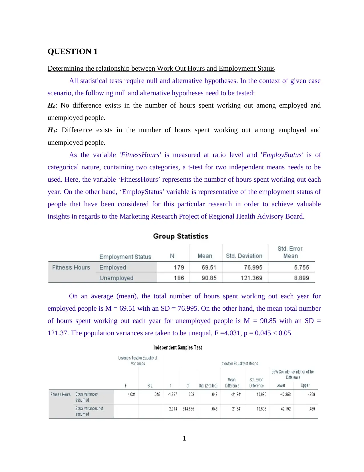
On an average (mean), the total number of hours spent working out each year for
employed people is M = 69.51 with an SD = 76.995. On the other hand, the mean total number
of hours spent working out each year for unemployed people is M = 90.85 with an SD =
121.37. The population variances are taken to be unequal, F =4.031, p = 0.045 < 0.05.
1
Determining the relationship between Work Out Hours and Employment Status
All statistical tests require null and alternative hypotheses. In the context of given case
scenario, the following null and alternative hypotheses need to be tested:
H0: No difference exists in the number of hours spent working out among employed and
unemployed people.
H1: Difference exists in the number of hours spent working out among employed and
unemployed people.
As the variable 'FitnessHours' is measured at ratio level and 'EmployStatus' is of
categorical nature, containing two categories, a t-test for two independent means needs to be
used. Here, the variable ‘FitnessHours’ represents the number of hours spent working out each
year. On the other hand, ‘EmployStatus’ variable is representative of the employment status of
people that have been considered for this particular research in order to achieve valuable
insights in regards to the Marketing Research Project of Regional Health Advisory Board.
On an average (mean), the total number of hours spent working out each year for
employed people is M = 69.51 with an SD = 76.995. On the other hand, the mean total number
of hours spent working out each year for unemployed people is M = 90.85 with an SD =
121.37. The population variances are taken to be unequal, F =4.031, p = 0.045 < 0.05.
1
⊘ This is a preview!⊘
Do you want full access?
Subscribe today to unlock all pages.
Trusted by 1+ million students worldwide
It is important to note that Levene's Test for Equality of Variances requires homogenity
of variances while undertaking an Independent Samples Test. The t-statistic has a degree of
freedom of df = 314.855 for 'Fitness Hours' where Equal variances are assumed and df= -2.014
wherein equal variances are not assumed. This difference occurs mainly due to the manner in
which these values have been calculated (Cronk, 2017). On the other hand the p = .045 < .05
wherein equal Variances are not assumed, which means that the null hypothesis is rejected
(H0) and Alternative Hypothesis stands accepted (H1). Hence, based on the p-value, it can be
claimed that the number of hours spent working out each year differs significantly between
employed and unemployed, at the 0.05 significance level.
QUESTION 2
Association between Total Personal Income and Gambling Expenditure
In the context of given case scenario, the following null and alternative hypotheses need
to be tested:
H0: No association exists between a individual's total personal income and expenditure incurred
on gambling activities by them.
H1: An association exists between a individual's total personal income and expenditure
incurred on gambling activities by them.
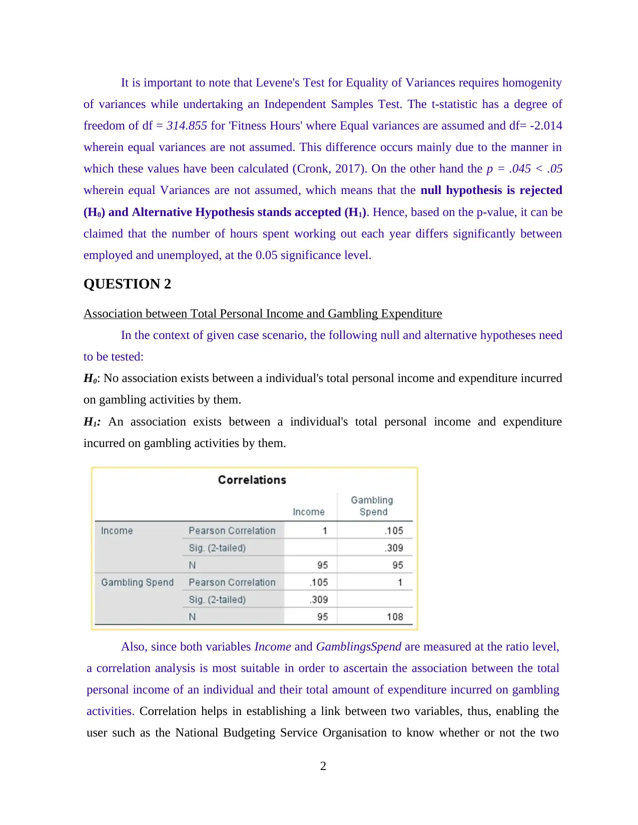
Also, since both variables Income and GamblingsSpend are measured at the ratio level,
a correlation analysis is most suitable in order to ascertain the association between the total
personal income of an individual and their total amount of expenditure incurred on gambling
activities. Correlation helps in establishing a link between two variables, thus, enabling the
user such as the National Budgeting Service Organisation to know whether or not the two
2
of variances while undertaking an Independent Samples Test. The t-statistic has a degree of
freedom of df = 314.855 for 'Fitness Hours' where Equal variances are assumed and df= -2.014
wherein equal variances are not assumed. This difference occurs mainly due to the manner in
which these values have been calculated (Cronk, 2017). On the other hand the p = .045 < .05
wherein equal Variances are not assumed, which means that the null hypothesis is rejected
(H0) and Alternative Hypothesis stands accepted (H1). Hence, based on the p-value, it can be
claimed that the number of hours spent working out each year differs significantly between
employed and unemployed, at the 0.05 significance level.
QUESTION 2
Association between Total Personal Income and Gambling Expenditure
In the context of given case scenario, the following null and alternative hypotheses need
to be tested:
H0: No association exists between a individual's total personal income and expenditure incurred
on gambling activities by them.
H1: An association exists between a individual's total personal income and expenditure
incurred on gambling activities by them.
Also, since both variables Income and GamblingsSpend are measured at the ratio level,
a correlation analysis is most suitable in order to ascertain the association between the total
personal income of an individual and their total amount of expenditure incurred on gambling
activities. Correlation helps in establishing a link between two variables, thus, enabling the
user such as the National Budgeting Service Organisation to know whether or not the two
2
Paraphrase This Document
Need a fresh take? Get an instant paraphrase of this document with our AI Paraphraser
variables impact each other in a certain way or not. Also, it helps in ascertaining whether this
relationship is strong enough to adversely impact the progress of these two variables.
As per the above results, it can be seen that the correlation between the Income and
Gambling Spend = 0.105 at a p-value = 0.309 > 0.05 under the Pearson's Correlation
Methodology. As per this methodology, a value above 0.5 states that there is a significant
association between the two variables being taken into consideration (Hinton, McMurray and
Brownlow, 2014). Since this value is less than 0.5 and is positive in nature, it can be affirmed
confidently that there is a positive yet weak correlation between a person's total personal
income and the gambling activities they engage in, using a certain portion of their income on
such acts. Thus, indicating that there is no significant relationship between the two variables
under observation showing deprivation of sufficiency of evidence to claim there association
with each other.
Hence, one can reject the alternative hypothesis (H1) and reject the alternative
hypothesis (H1) which states that a person’s total personal income is associated with the level
of money spent on gambling.
QUESTION 3
Role of Age and Attitude in gaining a University Qualification
In the context of given case scenario, the following null and alternative hypotheses need
to be tested:
H0: No relationship exists between Age and Attitude toward gaining a University Qualification.
H1: A relationship exists between Age and Attitude toward gaining a University Qualification.
The variable 'Attitude' comprises a large amount of behavioural categories that are
relatively equally spaced. Due to this, Attitude can be used as an interval variable although it is
usually measured at the ordinal level (George and Mallery, 2016). Here, the main motive of
the researcher, that is the Tertiary Education Advisory Board, is to gain valuable insights on
the current attitudes within society toward gaining a university qualification. The advisory
board believes that a person’s attitude toward university qualifications will be influenced by
their age. Thus, an ANOVA Analysis enables the user such as the Tertiary Education Advisory
Board to know whether or not the two variables impact each other in a certain way or not.
Also, it helps in ascertaining whether this relationship is strong enough to adversely impact the
3
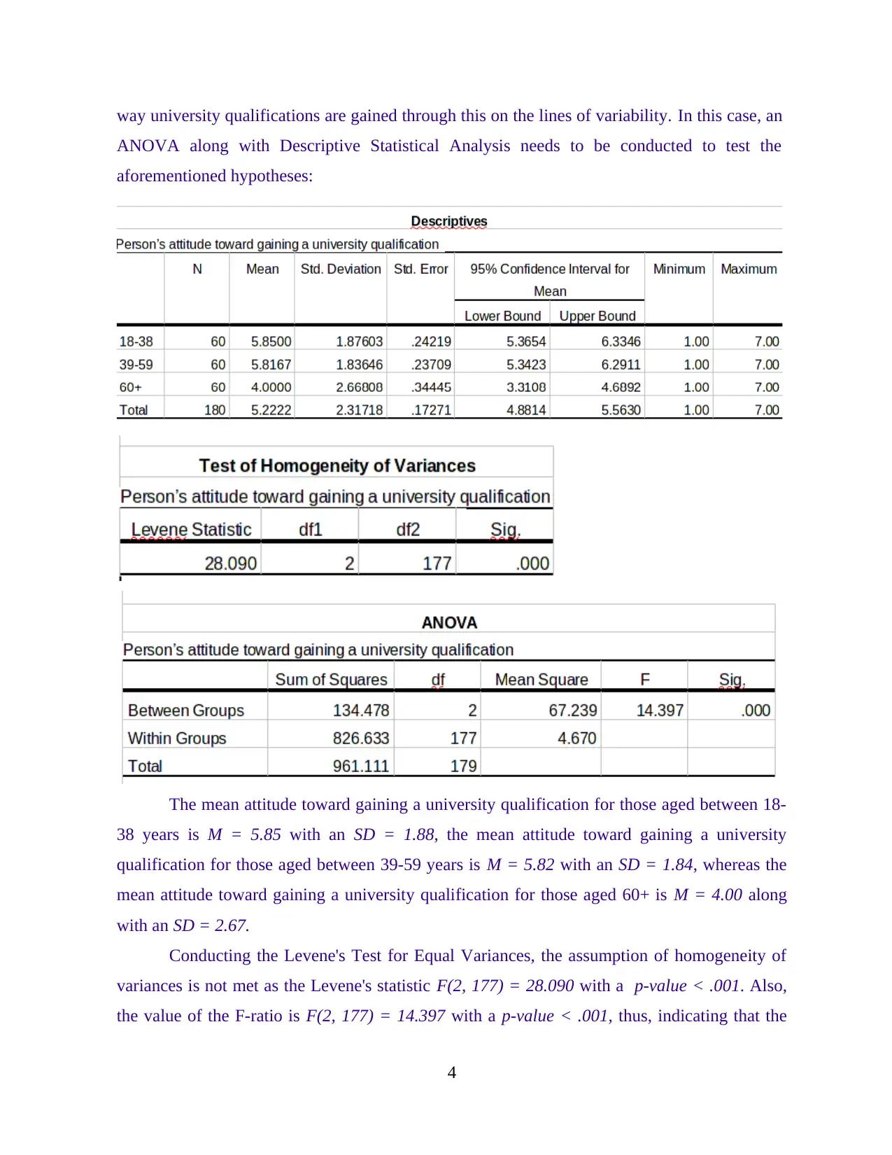
way university qualifications are gained through this on the lines of variability. In this case, an
ANOVA along with Descriptive Statistical Analysis needs to be conducted to test the
aforementioned hypotheses:
The mean attitude toward gaining a university qualification for those aged between 18-
38 years is M = 5.85 with an SD = 1.88, the mean attitude toward gaining a university
qualification for those aged between 39-59 years is M = 5.82 with an SD = 1.84, whereas the
mean attitude toward gaining a university qualification for those aged 60+ is M = 4.00 along
with an SD = 2.67.
Conducting the Levene's Test for Equal Variances, the assumption of homogeneity of
variances is not met as the Levene's statistic F(2, 177) = 28.090 with a p-value < .001. Also,
the value of the F-ratio is F(2, 177) = 14.397 with a p-value < .001, thus, indicating that the
4
⊘ This is a preview!⊘
Do you want full access?
Subscribe today to unlock all pages.
Trusted by 1+ million students worldwide
null hypothesis of equal means is rejected. Therefore, it can be asserted that there is
sufficient evidence to claim a relationship between age and attitude toward gaining a university
qualification.
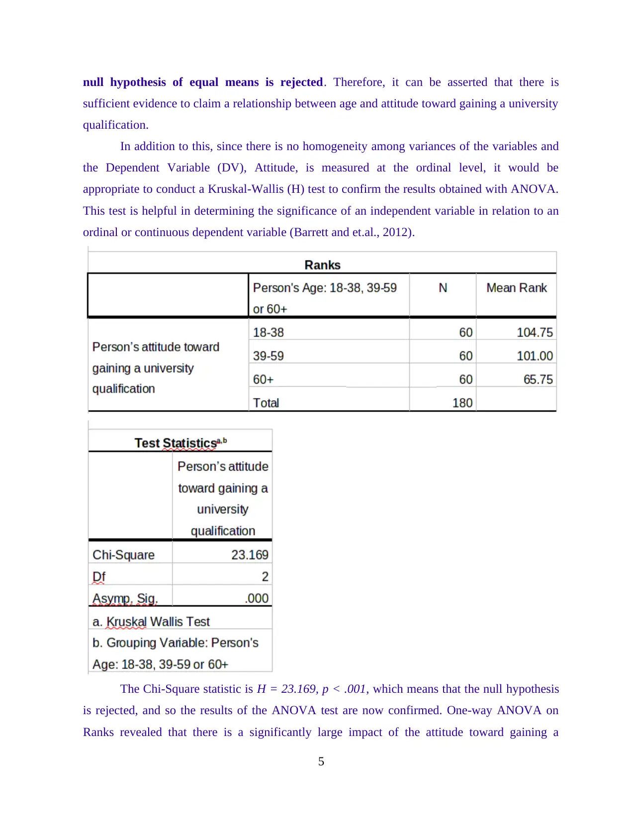
In addition to this, since there is no homogeneity among variances of the variables and
the Dependent Variable (DV), Attitude, is measured at the ordinal level, it would be
appropriate to conduct a Kruskal-Wallis (H) test to confirm the results obtained with ANOVA.
This test is helpful in determining the significance of an independent variable in relation to an
ordinal or continuous dependent variable (Barrett and et.al., 2012).
The Chi-Square statistic is H = 23.169, p < .001, which means that the null hypothesis
is rejected, and so the results of the ANOVA test are now confirmed. One-way ANOVA on
Ranks revealed that there is a significantly large impact of the attitude toward gaining a
5
sufficient evidence to claim a relationship between age and attitude toward gaining a university
qualification.
In addition to this, since there is no homogeneity among variances of the variables and
the Dependent Variable (DV), Attitude, is measured at the ordinal level, it would be
appropriate to conduct a Kruskal-Wallis (H) test to confirm the results obtained with ANOVA.
This test is helpful in determining the significance of an independent variable in relation to an
ordinal or continuous dependent variable (Barrett and et.al., 2012).
The Chi-Square statistic is H = 23.169, p < .001, which means that the null hypothesis
is rejected, and so the results of the ANOVA test are now confirmed. One-way ANOVA on
Ranks revealed that there is a significantly large impact of the attitude toward gaining a
5
Paraphrase This Document
Need a fresh take? Get an instant paraphrase of this document with our AI Paraphraser
university qualification at different age groups as F (2,177) =14.397, p<0.001. Meanwhile, H0
is rejected because p<0.05. There is a significant relationship between age and attitude toward
gaining a university qualification. Therefore, one can say that age is an important factor in
gaining University Qualification for an individual as it strongly impacts the attitude of that
person towards education as well as sense of achievement.
Hence, one can reject the null hypothesis (H0) and accept the alternative
hypothesis (H1) which states that a relationship exists between Age and Attitude toward
gaining a University Qualification.
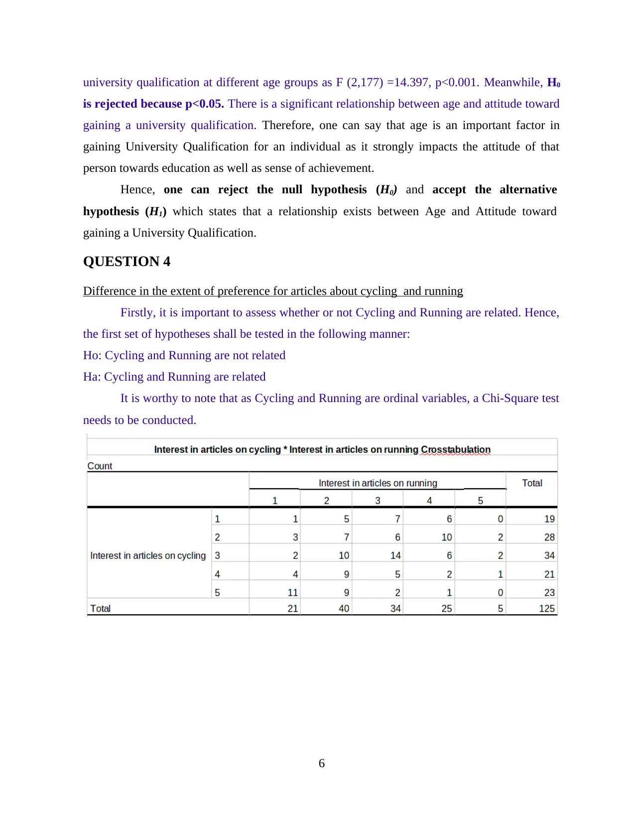
QUESTION 4
Difference in the extent of preference for articles about cycling and running
Firstly, it is important to assess whether or not Cycling and Running are related. Hence,
the first set of hypotheses shall be tested in the following manner:
Ho: Cycling and Running are not related
Ha: Cycling and Running are related
It is worthy to note that as Cycling and Running are ordinal variables, a Chi-Square test
needs to be conducted.
6
is rejected because p<0.05. There is a significant relationship between age and attitude toward
gaining a university qualification. Therefore, one can say that age is an important factor in
gaining University Qualification for an individual as it strongly impacts the attitude of that
person towards education as well as sense of achievement.
Hence, one can reject the null hypothesis (H0) and accept the alternative
hypothesis (H1) which states that a relationship exists between Age and Attitude toward
gaining a University Qualification.
QUESTION 4
Difference in the extent of preference for articles about cycling and running
Firstly, it is important to assess whether or not Cycling and Running are related. Hence,
the first set of hypotheses shall be tested in the following manner:
Ho: Cycling and Running are not related
Ha: Cycling and Running are related
It is worthy to note that as Cycling and Running are ordinal variables, a Chi-Square test
needs to be conducted.
6
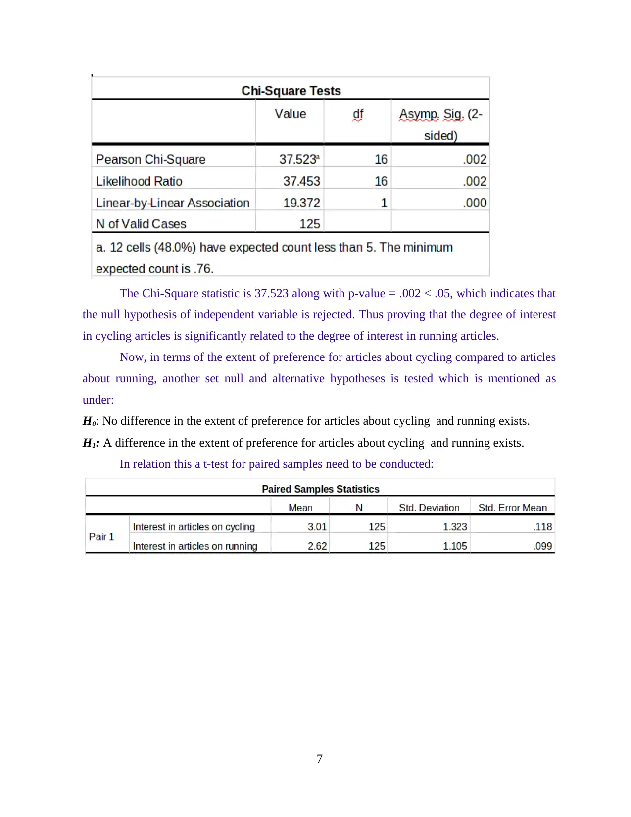
The Chi-Square statistic is 37.523 along with p-value = .002 < .05, which indicates that
the null hypothesis of independent variable is rejected. Thus proving that the degree of interest
in cycling articles is significantly related to the degree of interest in running articles.
Now, in terms of the extent of preference for articles about cycling compared to articles
about running, another set null and alternative hypotheses is tested which is mentioned as
under:
H0: No difference in the extent of preference for articles about cycling and running exists.
H1: A difference in the extent of preference for articles about cycling and running exists.
In relation this a t-test for paired samples need to be conducted:
7
⊘ This is a preview!⊘
Do you want full access?
Subscribe today to unlock all pages.
Trusted by 1+ million students worldwide
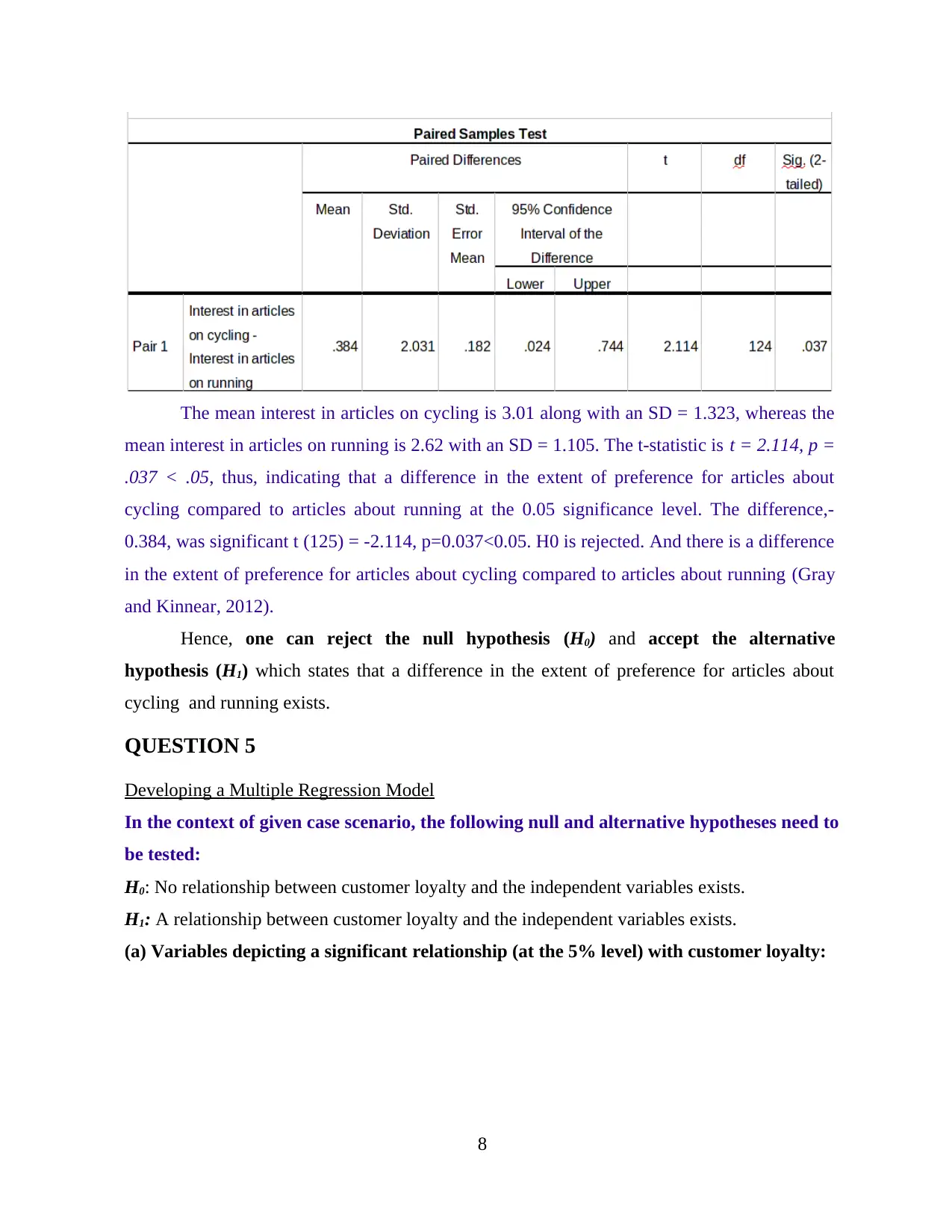
The mean interest in articles on cycling is 3.01 along with an SD = 1.323, whereas the
mean interest in articles on running is 2.62 with an SD = 1.105. The t-statistic is t = 2.114, p =
.037 < .05, thus, indicating that a difference in the extent of preference for articles about
cycling compared to articles about running at the 0.05 significance level. The difference,-
0.384, was significant t (125) = -2.114, p=0.037<0.05. H0 is rejected. And there is a difference
in the extent of preference for articles about cycling compared to articles about running (Gray
and Kinnear, 2012).
Hence, one can reject the null hypothesis (H0) and accept the alternative
hypothesis (H1) which states that a difference in the extent of preference for articles about
cycling and running exists.
QUESTION 5
Developing a Multiple Regression Model
In the context of given case scenario, the following null and alternative hypotheses need to
be tested:
H0: No relationship between customer loyalty and the independent variables exists.
H1: A relationship between customer loyalty and the independent variables exists.
(a) Variables depicting a significant relationship (at the 5% level) with customer loyalty:
8
Paraphrase This Document
Need a fresh take? Get an instant paraphrase of this document with our AI Paraphraser
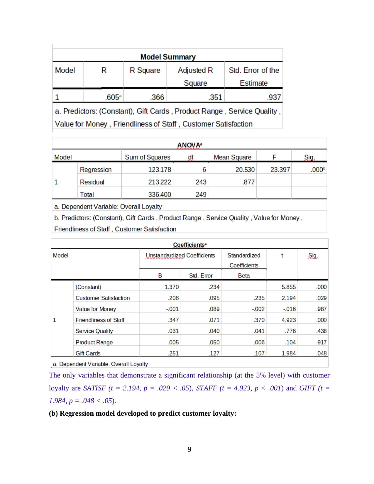
The only variables that demonstrate a significant relationship (at the 5% level) with customer
loyalty are SATISF (t = 2.194, p = .029 < .05), STAFF (t = 4.923, p < .001) and GIFT (t =
1.984, p = .048 < .05).
(b) Regression model developed to predict customer loyalty:
9
loyalty are SATISF (t = 2.194, p = .029 < .05), STAFF (t = 4.923, p < .001) and GIFT (t =
1.984, p = .048 < .05).
(b) Regression model developed to predict customer loyalty:
9
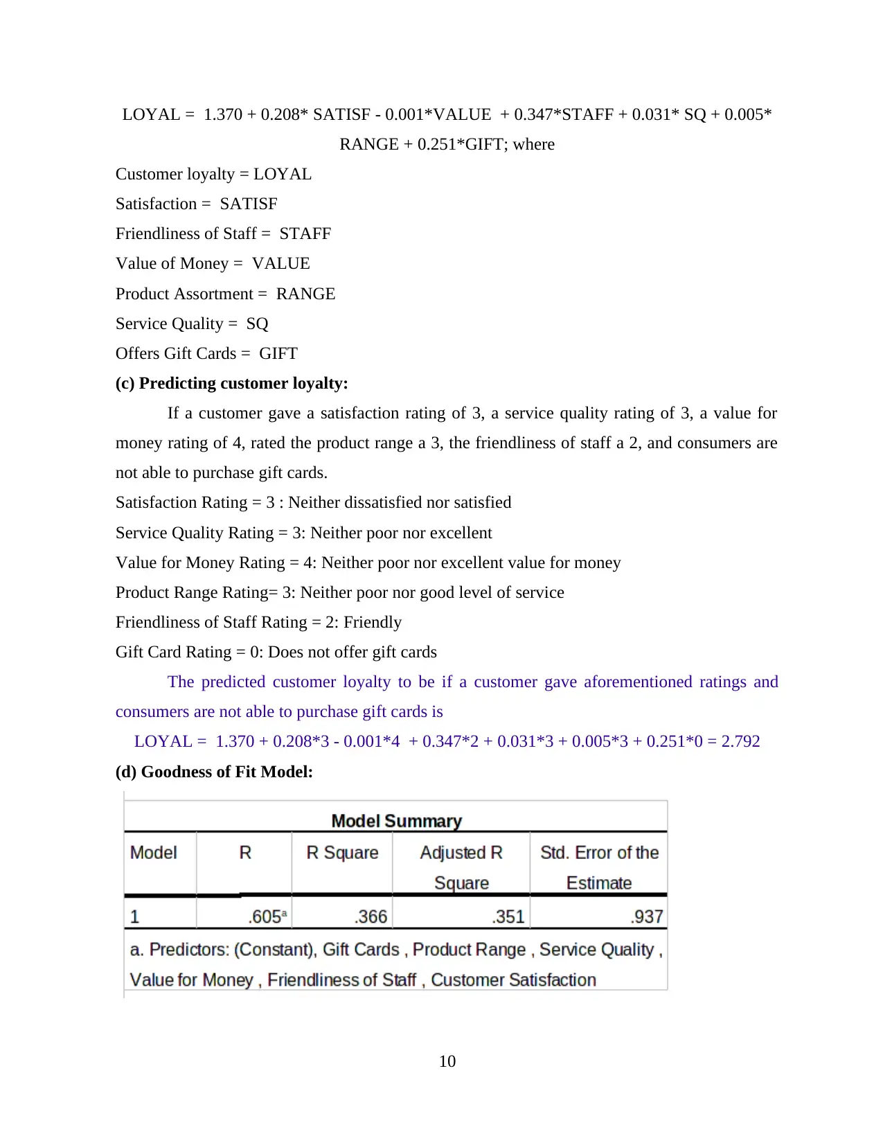
LOYAL = 1.370 + 0.208* SATISF - 0.001*VALUE + 0.347*STAFF + 0.031* SQ + 0.005*
RANGE + 0.251*GIFT; where
Customer loyalty = LOYAL
Satisfaction = SATISF
Friendliness of Staff = STAFF
Value of Money = VALUE
Product Assortment = RANGE
Service Quality = SQ
Offers Gift Cards = GIFT
(c) Predicting customer loyalty:
If a customer gave a satisfaction rating of 3, a service quality rating of 3, a value for
money rating of 4, rated the product range a 3, the friendliness of staff a 2, and consumers are
not able to purchase gift cards.
Satisfaction Rating = 3 : Neither dissatisfied nor satisfied
Service Quality Rating = 3: Neither poor nor excellent
Value for Money Rating = 4: Neither poor nor excellent value for money
Product Range Rating= 3: Neither poor nor good level of service
Friendliness of Staff Rating = 2: Friendly
Gift Card Rating = 0: Does not offer gift cards
The predicted customer loyalty to be if a customer gave aforementioned ratings and
consumers are not able to purchase gift cards is
LOYAL = 1.370 + 0.208*3 - 0.001*4 + 0.347*2 + 0.031*3 + 0.005*3 + 0.251*0 = 2.792
(d) Goodness of Fit Model:
10
⊘ This is a preview!⊘
Do you want full access?
Subscribe today to unlock all pages.
Trusted by 1+ million students worldwide
1 out of 14
Related Documents


Your All-in-One AI-Powered Toolkit for Academic Success.
+13062052269
info@desklib.com
Available 24*7 on WhatsApp / Email
![[object Object]](/_next/static/media/star-bottom.7253800d.svg)
Unlock your academic potential
Copyright © 2020–2026 A2Z Services. All Rights Reserved. Developed and managed by ZUCOL.