STA 250 SPSS Assignment: Statistical Analysis and Interpretation

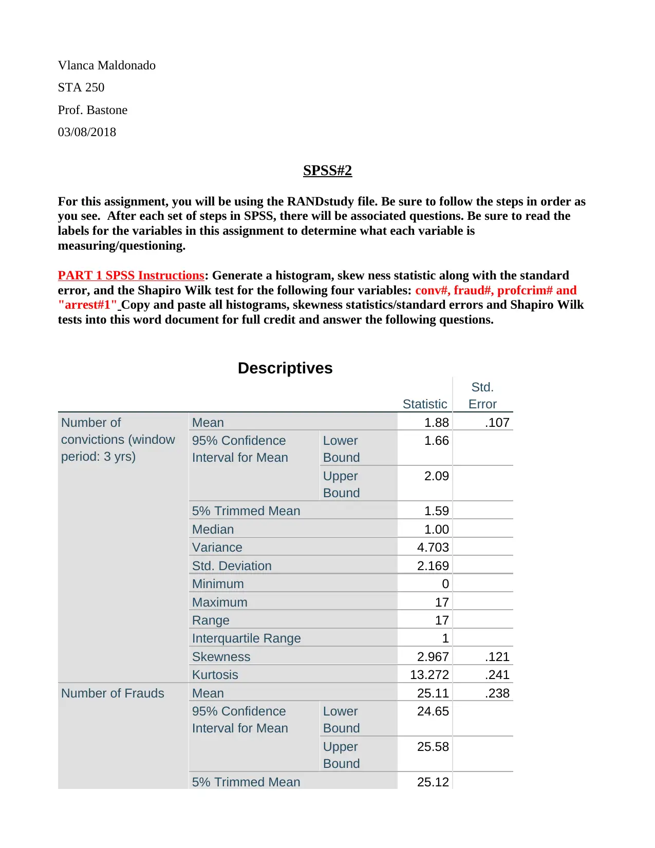
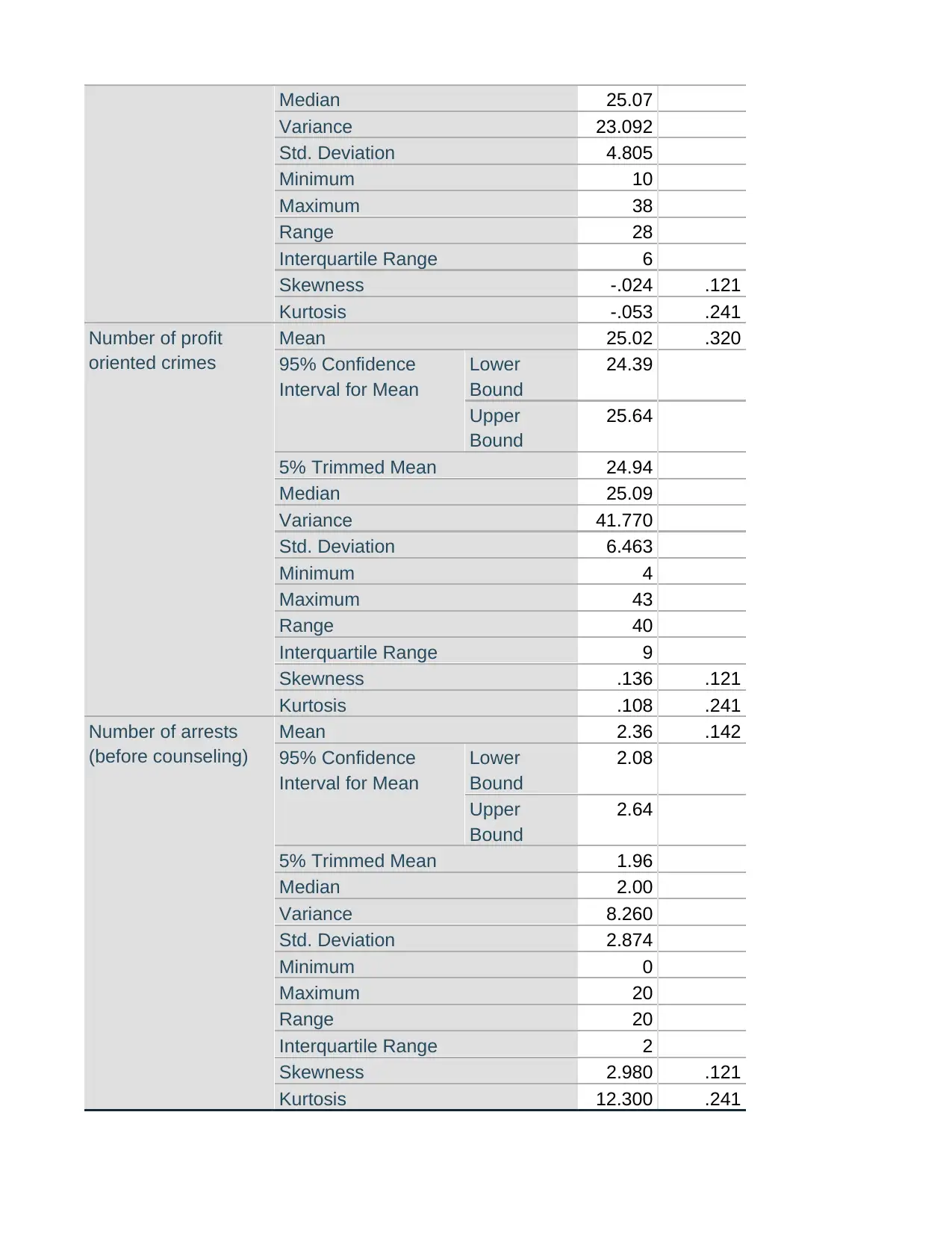
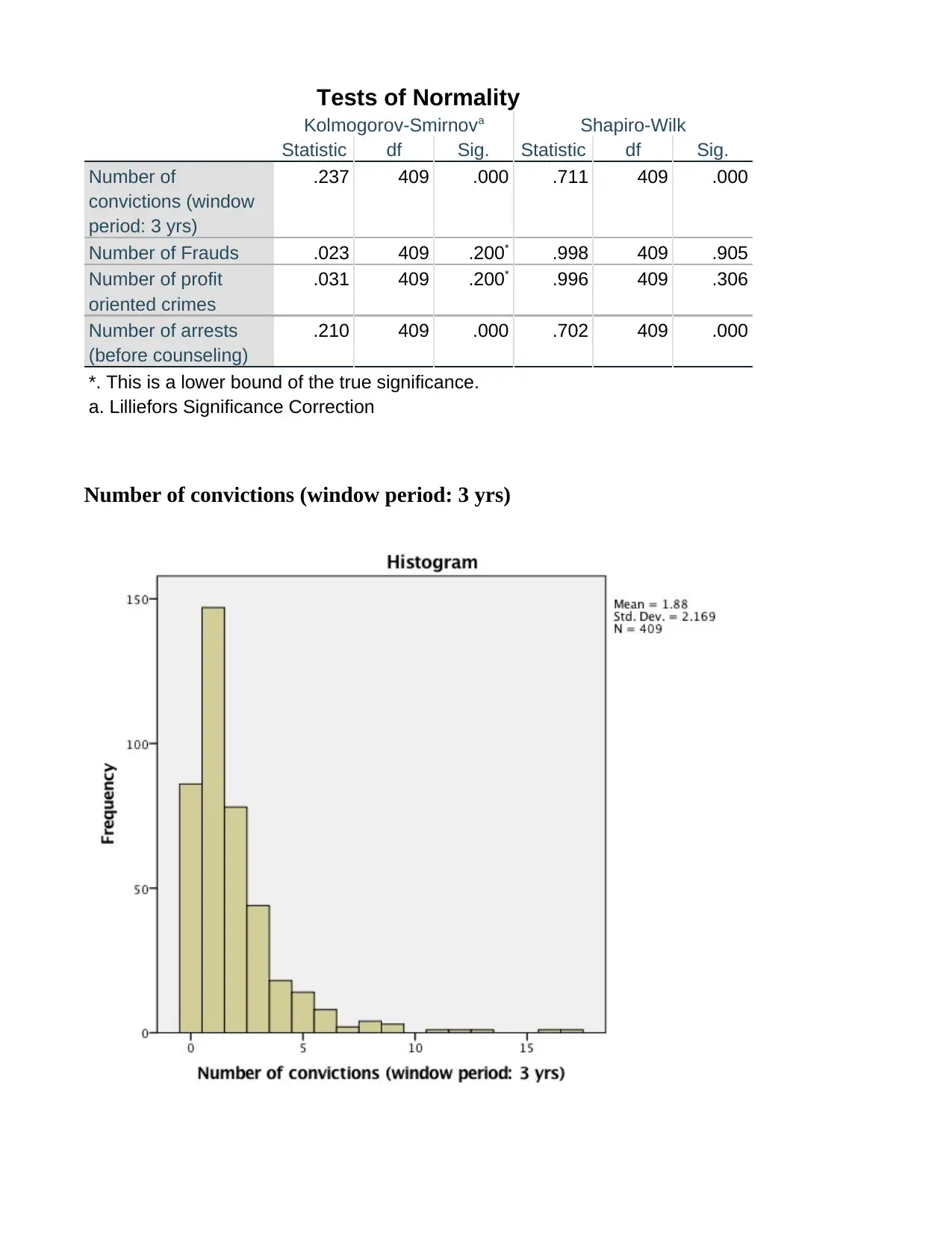
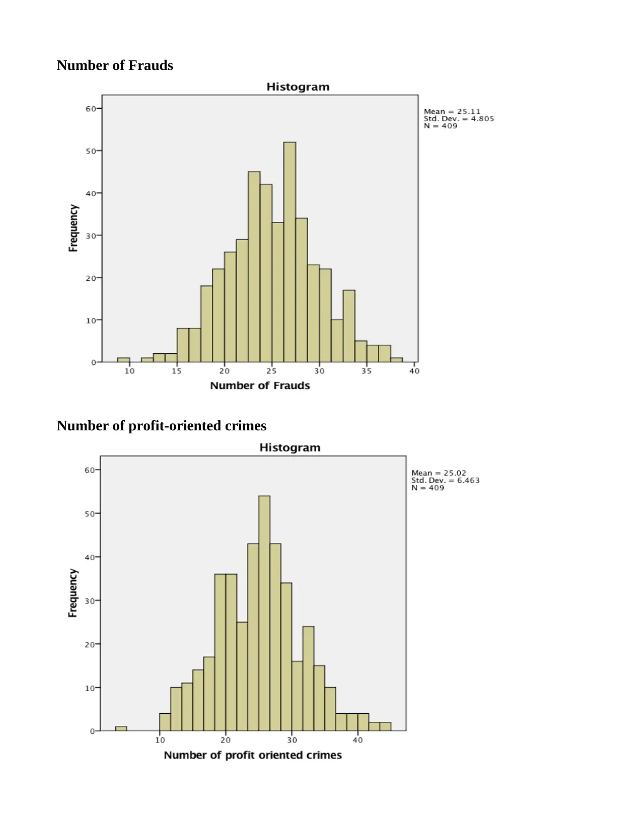
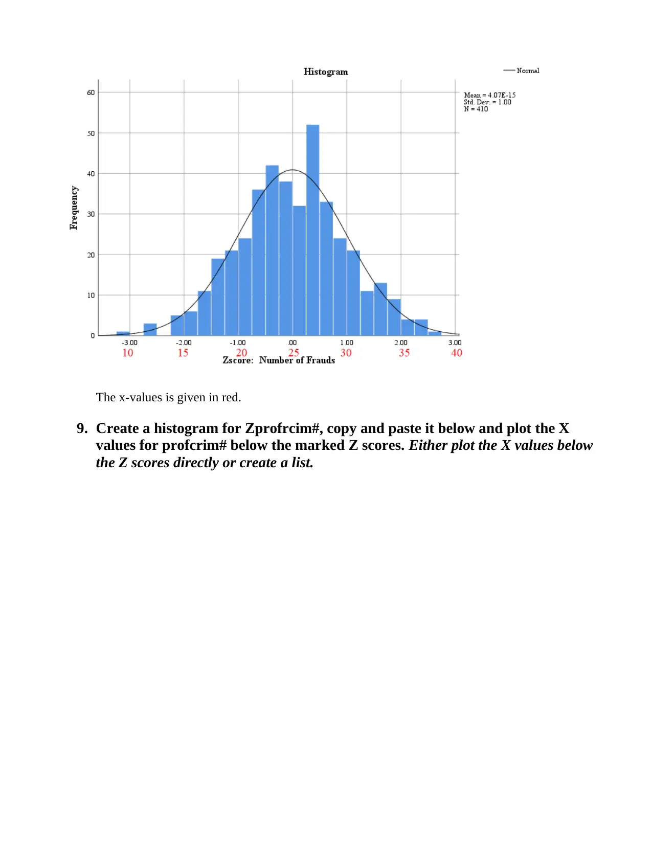
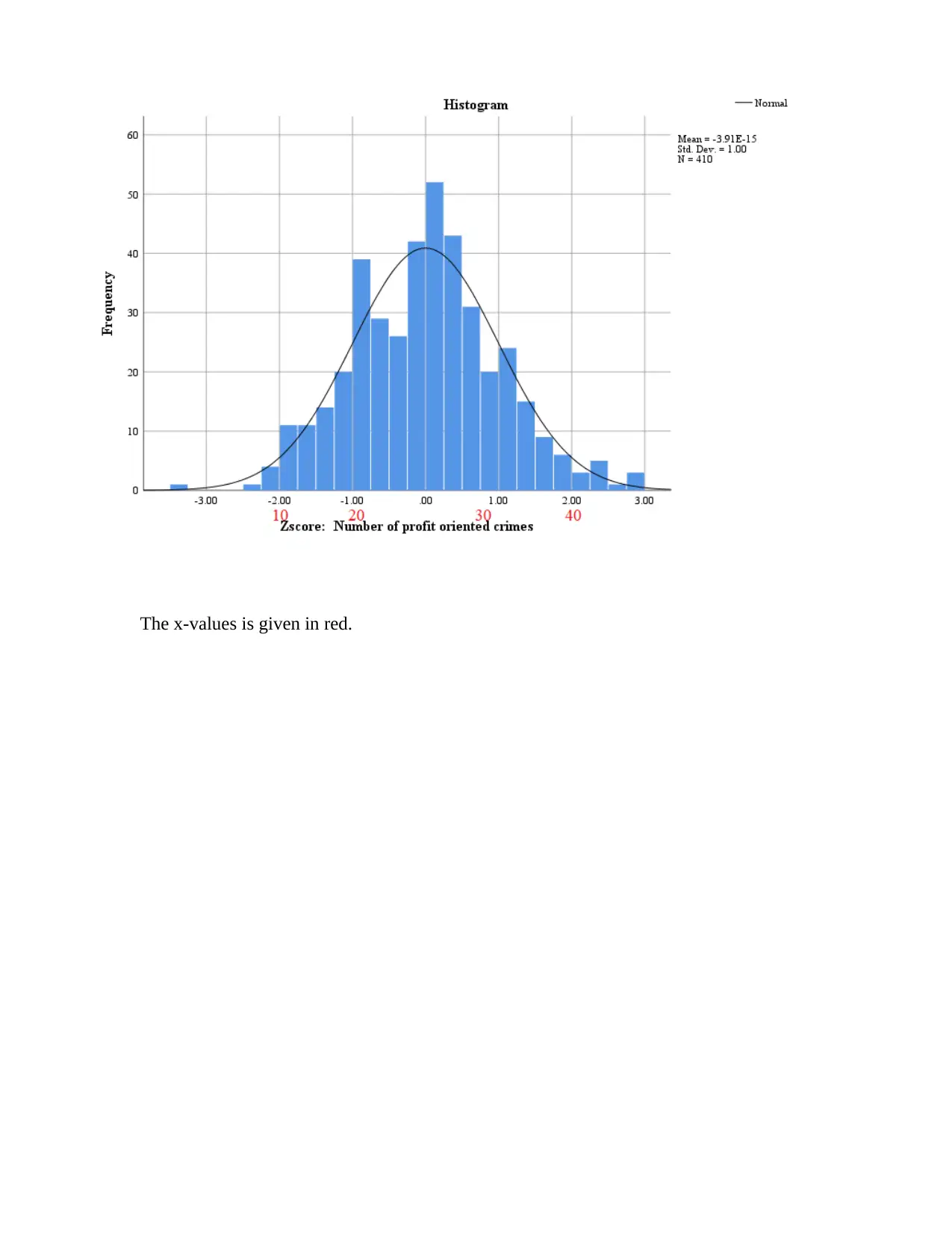
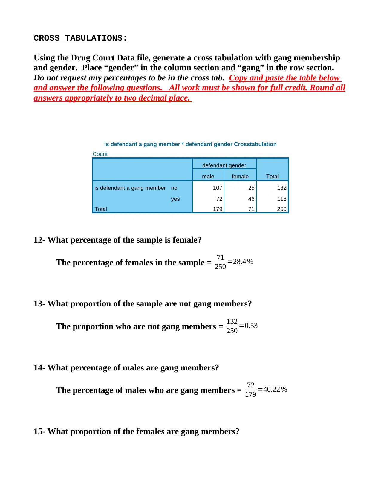
This SPSS assignment, completed by Vlanca Maldonado for STA 250, Prof. Bastone, covers various statistical concepts using the RANDstudy and Drug Court Data files. The assignment begins with generating histograms, calculating skewness, and performing the Shapiro-Wilk test for variables such as c...Read More

Vlanca Maldonado
STA 250
Prof. Bastone
03/08/2018
SPSS#2
For this assignment, you will be using the RANDstudy file. Be sure to follow the steps in order as
you see. After each set of steps in SPSS, there will be associated questions. Be sure to read the
labels for the variables in this assignment to determine what each variable is
measuring/questioning.
PART 1 SPSS Instructions: Generate a histogram, skew ness statistic along with the standard
error, and the Shapiro Wilk test for the following four variables: conv#, fraud#, profcrim# and
"arrest#1" Copy and paste all histograms, skewness statistics/standard errors and Shapiro Wilk
tests into this word document for full credit and answer the following questions.
Descriptives
Statistic
Std.
Error
Number of
convictions (window
period: 3 yrs)
Mean 1.88 .107
95% Confidence
Interval for Mean
Lower
Bound
1.66
Upper
Bound
2.09
5% Trimmed Mean 1.59
Median 1.00
Variance 4.703
Std. Deviation 2.169
Minimum 0
Maximum 17
Range 17
Interquartile Range 1
Skewness 2.967 .121
Kurtosis 13.272 .241
Number of Frauds Mean 25.11 .238
95% Confidence
Interval for Mean
Lower
Bound
24.65
Upper
Bound
25.58
5% Trimmed Mean 25.12

Median 25.07
Variance 23.092
Std. Deviation 4.805
Minimum 10
Maximum 38
Range 28
Interquartile Range 6
Skewness -.024 .121
Kurtosis -.053 .241
Number of profit
oriented crimes
Mean 25.02 .320
95% Confidence
Interval for Mean
Lower
Bound
24.39
Upper
Bound
25.64
5% Trimmed Mean 24.94
Median 25.09
Variance 41.770
Std. Deviation 6.463
Minimum 4
Maximum 43
Range 40
Interquartile Range 9
Skewness .136 .121
Kurtosis .108 .241
Number of arrests
(before counseling)
Mean 2.36 .142
95% Confidence
Interval for Mean
Lower
Bound
2.08
Upper
Bound
2.64
5% Trimmed Mean 1.96
Median 2.00
Variance 8.260
Std. Deviation 2.874
Minimum 0
Maximum 20
Range 20
Interquartile Range 2
Skewness 2.980 .121
Kurtosis 12.300 .241

Tests of Normality
Kolmogorov-Smirnova Shapiro-Wilk
Statistic df Sig. Statistic df Sig.
Number of
convictions (window
period: 3 yrs)
.237 409 .000 .711 409 .000
Number of Frauds .023 409 .200* .998 409 .905
Number of profit
oriented crimes
.031 409 .200* .996 409 .306
Number of arrests
(before counseling)
.210 409 .000 .702 409 .000
*. This is a lower bound of the true significance.
a. Lilliefors Significance Correction
Number of convictions (window period: 3 yrs)

Number of Frauds
Number of profit-oriented crimes

Number of arrests (before counseling)
1. From viewing the histogram, skew ness value/std. error and the results of the
Shapiro Wilk test, describe in at least six sentences total the shape of the
distribution for arrest# AND conv#. You should have three sentences for each
variable.
Arrest# The histogram for Arrests is skewed to the right. The skewness
data shows that the data for Arrests is positively skewed (2.980). From
the Shapiro-Wilk test it is found that the data is not normally
distributed (Sig = 0.000).
Conv# The shape of the histogram is skewed to the right. The data of
conv# is positively skewed (2.967). From the Shapiro-Wilk test it is
found that the data is not normally distributed (Sig = 0.000).
2. From viewing the histogram, skew ness value/ std. error and the results of the
Shapiro Wilk test, describe in at least six sentence total the shape of the
distribution for profcrim# and fraud#. You should have three sentences for
each variable.

Fraud# The shape of the histogram is approximately normally
distributed. The data of Fraud# is approximately normal since it is close
to zero (-0.024). From the Shapiro-Wilk test it is found that the data is
normally distributed (Sig = 0.905).
Profcrim# The shape of the histogram is approximately normally
distributed. The data for number of profit oriented crime is
approximately normal (0.136). From the Shapiro-Wilk test it is found
that the data is not normally distributed (Sig = 0.306).
3. Of the four variables you just described in questions 1 and 2, which ones are
appropriate to create Z scores for? Write “NA” if not appropriate write “A”
if appropriate.
Profcrim# A
Fraud# A
Arrest# A
Conv# A
4. From viewing the X value histogram for “FRAUD#”, indicate the
highest/maximum X value- your answer is somewhat estimated. (this is not the
X value with the highest frequency). Where would you expect that X value be
in the Z distribution for ZFRAUD#? You can give a general location or
actually calculate the Z score and give an exact location. Show any
mathematical work for full credit.
Highest/Maximum X value The maximum value for FRAUD# is 27
Associated Z score (General location)
__________________________________________________________________
_____________
OR
Associated Z score (Specific location)

The mean for FRAUD# is 25.10 and standard deviation is 4.813
Hence the associated Z-score for highest FRAUD# = 27−25.10
4.813 =0.39
5. From viewing the X value histogram for profcrim#, report the
lowest/minimum X value- this is somewhat estimated (again, this is not the
value with the lowest frequency). Where would you expect that to be in the Z
distribution for Zprofcrim#? Either give a general location or actually
calculate the Z score and report an exact location. Show any math work for full
credit.
Lowest X value The minimum value for profcrim is 4
Associated Z score (General
location___________________________________________________________
OR
Associated Z score (Specific location)______________________Show work.
The mean for profcrim is 25.00 and standard deviation is 6.467
Hence the associated Z-score for highest profcrim = 4−25.00
6.467 =−3.65
6. From viewing the X value histogram for fraud#, report the average. Where
would that value be as a Z score in Zfraud#?
Average 25.11
Z score location =0.00

Part 2 SPSS Instructions: Create Z scores for "profcrim#" & "fraud#" Then,
after the Z score variables are created, create a set of descriptive statistics for
both Z score variables (Zprofcrim# & Zfraud#), both Zscore variables should
have the- mean, standard deviation, minimum and maximum value. You also
need create a set of descriptive statistics (mean, standard deviation, minimum
and maximum value) for the associated X value variables: profcrim# and
fraud#. Copy and paste the four sets of descriptive statistics below for full
credit.
7. Why do the X value variables, “profcrim#” & “fraud#" have a different mean
and standard deviation than their associated Zscore variables, “Zprofcrim#”
& “Zfraud#”? Answer should be at least 3-4 sentences.
The mean and standard deviation of the variables of profcrim# and fraud# are calculated taking
into consideration all the values. Whereas, the z-value is based on the location of the x-value
corresponding to the mean and standard deviation. Hence, all x-values which are below the mean
of the concerned variable would be negative while all above the mean would be positive.
8. Create a histogram for Zfraud#, copy and paste it below and plot the X values
for fraud below the marked Z scores using the mean and standard deviation
from the X value variable. If you cannot get each X value below the Z score
directly, you can just create an organized list anywhere below the chart.

The x-values is given in red.
9. Create a histogram for Zprofrcim#, copy and paste it below and plot the X
values for profcrim# below the marked Z scores. Either plot the X values below
the Z scores directly or create a list.

The x-values is given in red.

CROSS TABULATIONS:
Using the Drug Court Data file, generate a cross tabulation with gang membership
and gender. Place “gender” in the column section and “gang” in the row section.
Do not request any percentages to be in the cross tab. Copy and paste the table below
and answer the following questions. All work must be shown for full credit. Round all
answers appropriately to two decimal place.
is defendant a gang member * defendant gender Crosstabulation
Count
defendant gender
Totalmale female
is defendant a gang member no 107 25 132
yes 72 46 118
Total 179 71 250
12- What percentage of the sample is female?
The percentage of females in the sample = 71
250 =28.4 %
13- What proportion of the sample are not gang members?
The proportion who are not gang members = 132
250 =0.53
14- What percentage of males are gang members?
The percentage of males who are gang members = 72
179 =40.22 %
15- What proportion of the females are gang members?

The proportion of female who are gang members = 46
71 =0.65
16- What percentage of non- gang members are male?
The percentage of non-gang members who are males = 107
132 =81.06 %
17- Which gender is more likely to be in a gang? Explain using probabilities.
The probability of female being in gang is 0.65 while for male is 0.40. Thus a
female is more likely to be in gang.
18- Does it appear that gender influences gang membership? Explain using
probabilities
The probability that a gang member is a male = 0.61.
The probability that a gang member is a female = 0.39
Since, the probability that a gang member is a male is higher that of female,
hence it seems that gender influences gang membership.