SPSS Statistics Assignment: Test Scores, Gender, and Program
VerifiedAdded on 2023/01/17
|42
|9930
|50
Homework Assignment
AI Summary
This SPSS assignment analyzes test scores of low-income students participating in an afterschool program. The assignment explores three key questions. First, it investigates if there are significant differences between the practice test scores of these students and state averages across reading, math, and science. One-sample t-tests are used to compare sample means to known population values. Second, it examines whether student test scores improved over time in reading, math, and science, employing paired t-tests to compare scores at the beginning and later in the year. Finally, the assignment investigates the presence of gender differences in math, science, and reading scores, using independent samples t-tests to compare the means of male and female students. The assignment includes the hypotheses, statistical tests, and the interpretation of results with statistical outputs.

SPSS Statistics Assignment
Student Name:
Instructor Name:
Course Number:
10 April 2019
Student Name:
Instructor Name:
Course Number:
10 April 2019
Paraphrase This Document
Need a fresh take? Get an instant paraphrase of this document with our AI Paraphraser
Question 1: Is there a significant difference between the practice test scores of low income
students participating in the afterschool program and the state averages in each test area?
For this question, we sought to test three different hypotheses. The hypotheses are given as
follows;
Hypothesis 1:
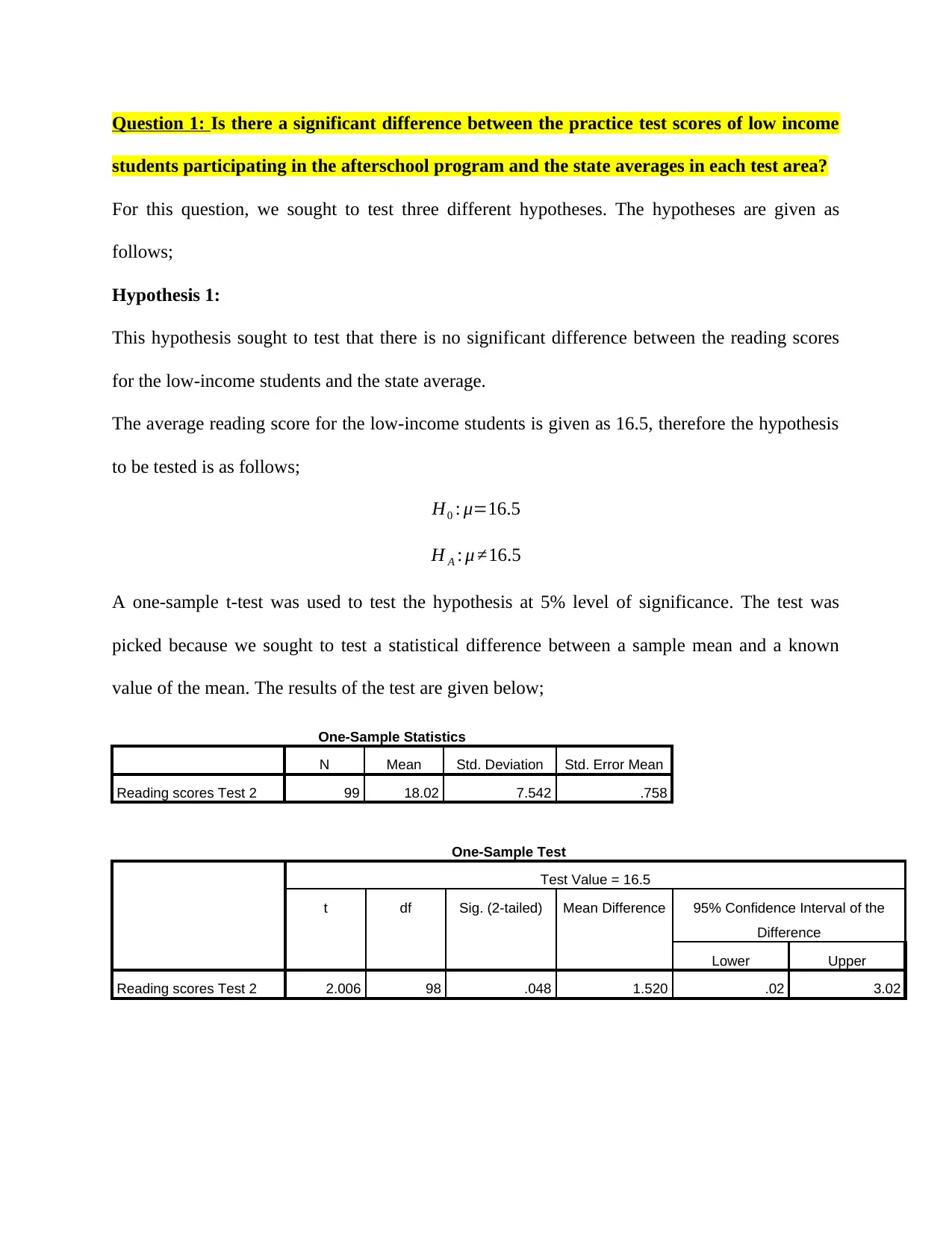
This hypothesis sought to test that there is no significant difference between the reading scores
for the low-income students and the state average.
The average reading score for the low-income students is given as 16.5, therefore the hypothesis
to be tested is as follows;
H0 : μ=16.5
H A : μ ≠16.5
A one-sample t-test was used to test the hypothesis at 5% level of significance. The test was
picked because we sought to test a statistical difference between a sample mean and a known
value of the mean. The results of the test are given below;
One-Sample Statistics
N Mean Std. Deviation Std. Error Mean
Reading scores Test 2 99 18.02 7.542 .758
One-Sample Test
Test Value = 16.5
t df Sig. (2-tailed) Mean Difference 95% Confidence Interval of the
Difference
Lower Upper
Reading scores Test 2 2.006 98 .048 1.520 .02 3.02
students participating in the afterschool program and the state averages in each test area?
For this question, we sought to test three different hypotheses. The hypotheses are given as
follows;
Hypothesis 1:
This hypothesis sought to test that there is no significant difference between the reading scores
for the low-income students and the state average.
The average reading score for the low-income students is given as 16.5, therefore the hypothesis
to be tested is as follows;
H0 : μ=16.5
H A : μ ≠16.5
A one-sample t-test was used to test the hypothesis at 5% level of significance. The test was
picked because we sought to test a statistical difference between a sample mean and a known
value of the mean. The results of the test are given below;
One-Sample Statistics
N Mean Std. Deviation Std. Error Mean
Reading scores Test 2 99 18.02 7.542 .758
One-Sample Test
Test Value = 16.5
t df Sig. (2-tailed) Mean Difference 95% Confidence Interval of the
Difference
Lower Upper
Reading scores Test 2 2.006 98 .048 1.520 .02 3.02
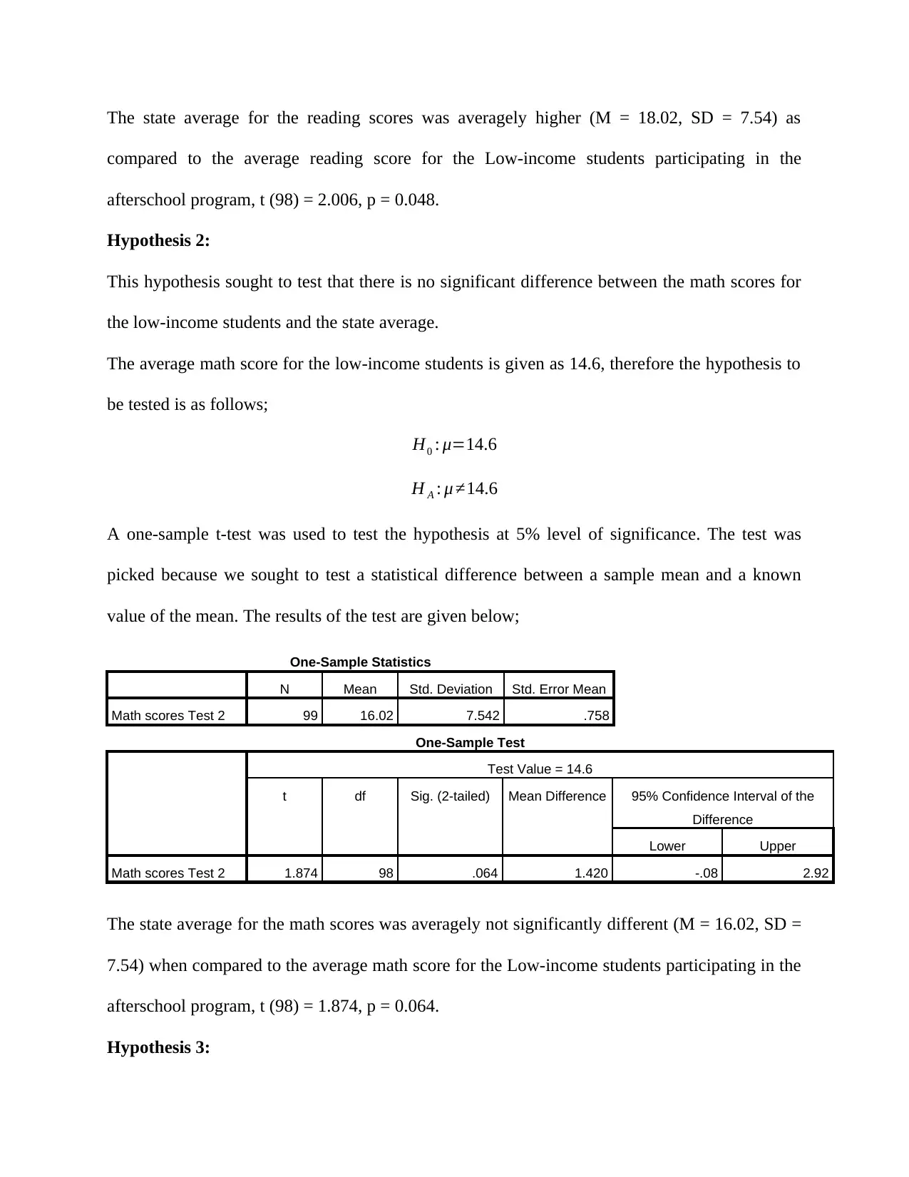
The state average for the reading scores was averagely higher (M = 18.02, SD = 7.54) as
compared to the average reading score for the Low-income students participating in the
afterschool program, t (98) = 2.006, p = 0.048.
Hypothesis 2:
This hypothesis sought to test that there is no significant difference between the math scores for
the low-income students and the state average.
The average math score for the low-income students is given as 14.6, therefore the hypothesis to
be tested is as follows;
H0 : μ=14.6
H A : μ ≠14.6
A one-sample t-test was used to test the hypothesis at 5% level of significance. The test was
picked because we sought to test a statistical difference between a sample mean and a known
value of the mean. The results of the test are given below;
One-Sample Statistics
N Mean Std. Deviation Std. Error Mean
Math scores Test 2 99 16.02 7.542 .758
One-Sample Test
Test Value = 14.6
t df Sig. (2-tailed) Mean Difference 95% Confidence Interval of the
Difference
Lower Upper
Math scores Test 2 1.874 98 .064 1.420 -.08 2.92
The state average for the math scores was averagely not significantly different (M = 16.02, SD =
7.54) when compared to the average math score for the Low-income students participating in the
afterschool program, t (98) = 1.874, p = 0.064.
Hypothesis 3:
⊘ This is a preview!⊘
Do you want full access?
Subscribe today to unlock all pages.
Trusted by 1+ million students worldwide
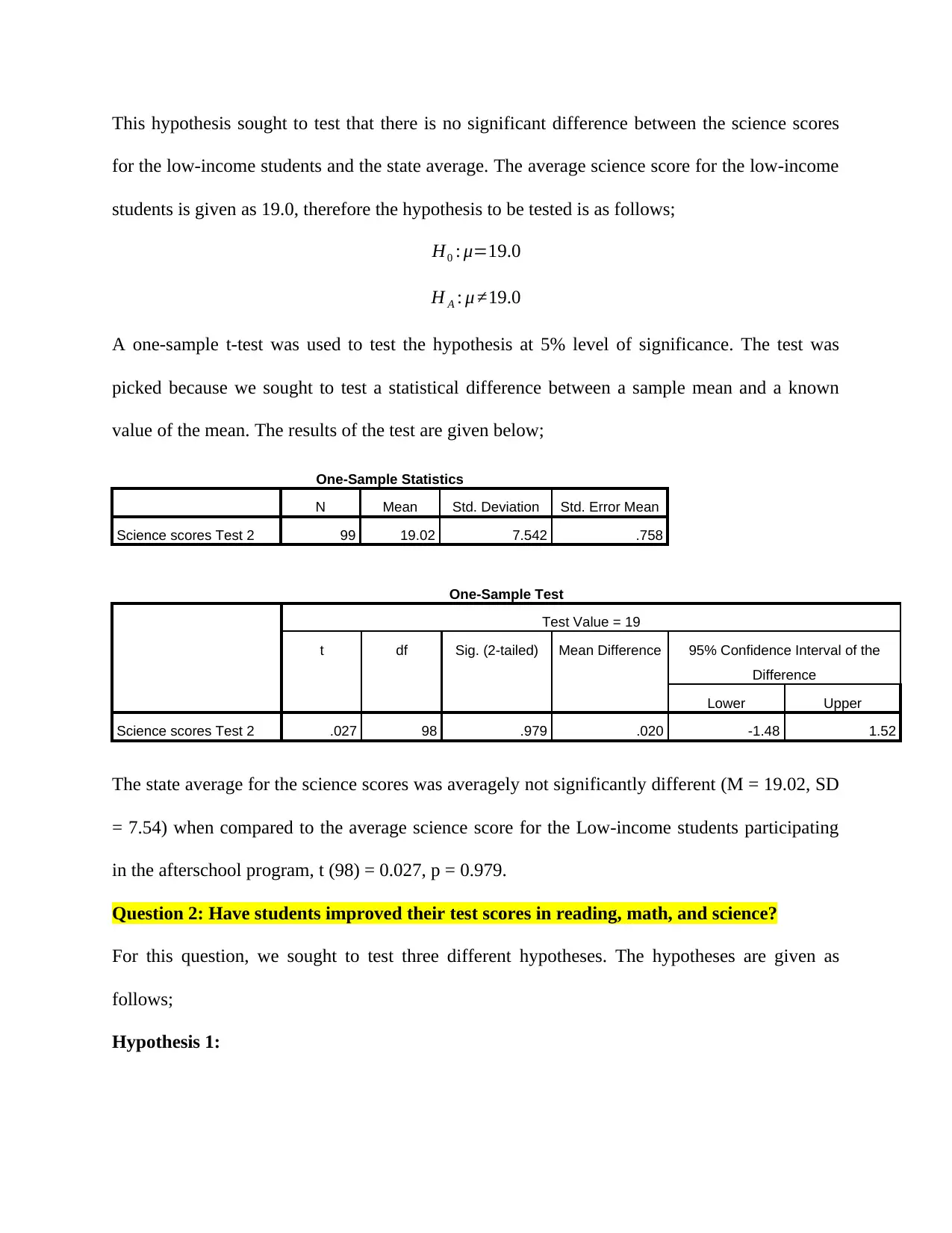
This hypothesis sought to test that there is no significant difference between the science scores
for the low-income students and the state average. The average science score for the low-income
students is given as 19.0, therefore the hypothesis to be tested is as follows;
H0 : μ=19.0
H A : μ ≠19.0
A one-sample t-test was used to test the hypothesis at 5% level of significance. The test was
picked because we sought to test a statistical difference between a sample mean and a known
value of the mean. The results of the test are given below;
One-Sample Statistics
N Mean Std. Deviation Std. Error Mean
Science scores Test 2 99 19.02 7.542 .758
One-Sample Test
Test Value = 19
t df Sig. (2-tailed) Mean Difference 95% Confidence Interval of the
Difference
Lower Upper
Science scores Test 2 .027 98 .979 .020 -1.48 1.52
The state average for the science scores was averagely not significantly different (M = 19.02, SD
= 7.54) when compared to the average science score for the Low-income students participating
in the afterschool program, t (98) = 0.027, p = 0.979.
Question 2: Have students improved their test scores in reading, math, and science?
For this question, we sought to test three different hypotheses. The hypotheses are given as
follows;
Hypothesis 1:
Paraphrase This Document
Need a fresh take? Get an instant paraphrase of this document with our AI Paraphraser
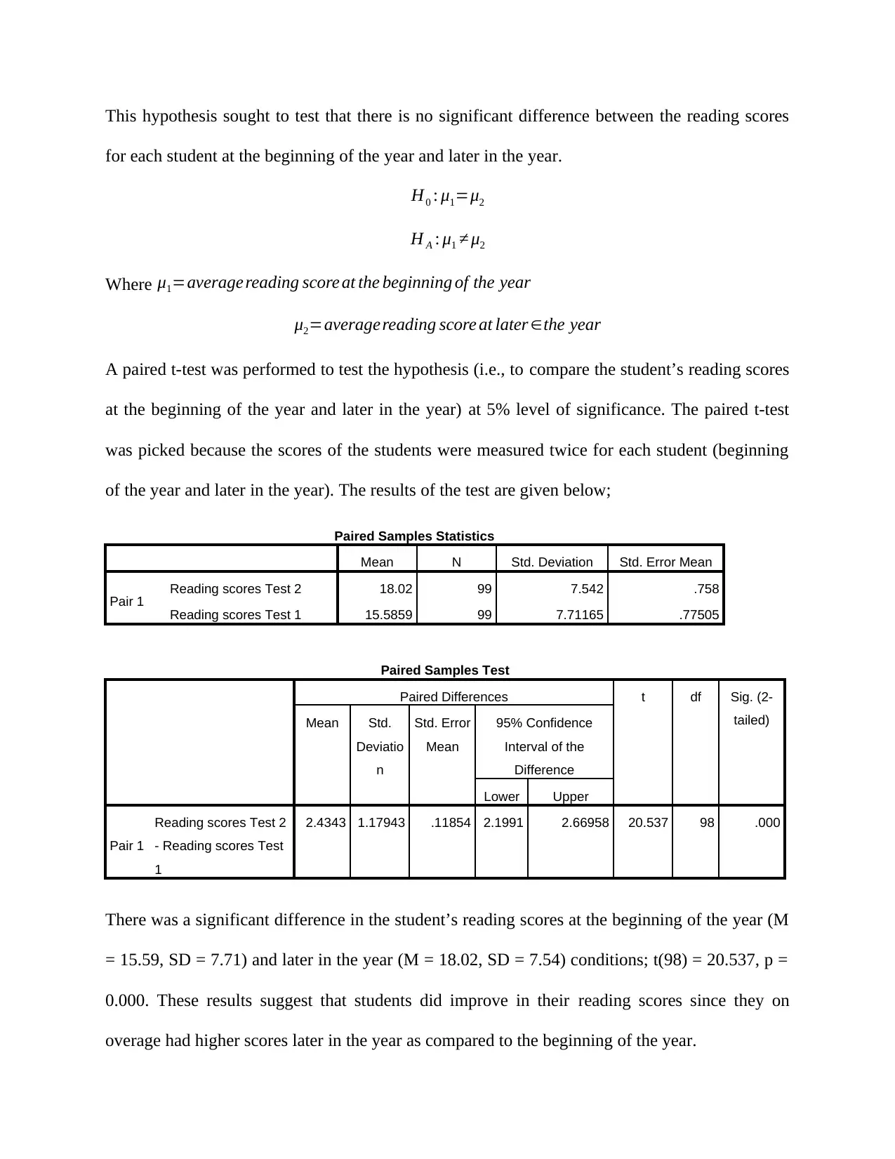
This hypothesis sought to test that there is no significant difference between the reading scores
for each student at the beginning of the year and later in the year.
H0 : μ1=μ2
H A : μ1 ≠ μ2
Where μ1=average reading score at the beginning of the year
μ2=averagereading score at later ∈the year
A paired t-test was performed to test the hypothesis (i.e., to compare the student’s reading scores
at the beginning of the year and later in the year) at 5% level of significance. The paired t-test
was picked because the scores of the students were measured twice for each student (beginning
of the year and later in the year). The results of the test are given below;
Paired Samples Statistics
Mean N Std. Deviation Std. Error Mean
Pair 1 Reading scores Test 2 18.02 99 7.542 .758
Reading scores Test 1 15.5859 99 7.71165 .77505
Paired Samples Test
Paired Differences t df Sig. (2-
tailed)Mean Std.
Deviatio
n
Std. Error
Mean
95% Confidence
Interval of the
Difference
Lower Upper
Pair 1
Reading scores Test 2
- Reading scores Test
1
2.4343 1.17943 .11854 2.1991 2.66958 20.537 98 .000
There was a significant difference in the student’s reading scores at the beginning of the year (M
= 15.59, SD = 7.71) and later in the year (M = 18.02, SD = 7.54) conditions; t(98) = 20.537, p =
0.000. These results suggest that students did improve in their reading scores since they on
overage had higher scores later in the year as compared to the beginning of the year.
Hypothesis 2:
This hypothesis sought to test that there is no significant difference between the math scores for
each student at the beginning of the year and later in the year.
H0 : μ1=μ2
H A : μ1 ≠ μ2
Where μ1=average math score at the beginning of the year
μ2=average math score at later ∈the year
A paired t-test was performed to test the hypothesis (i.e., to compare the student’s math scores at
the beginning of the year and later in the year) at 5% level of significance. The paired t-test was
picked because the scores of the students were measured twice for each student (beginning of the
year and later in the year). The results of the test are given below;
Paired Samples Statistics
Mean N Std. Deviation Std. Error Mean
Pair 1 Math scores Test 2 16.02 99 7.542 .758
Math scores Test 1 13.5051 99 7.64436 .76829
Paired Samples Test
Paired Differences t df Sig. (2-
tailed)Mean Std.
Deviation
Std. Error
Mean
95% Confidence
Interval of the
Difference
Lower Upper
Pair
1
Math scores Test 2
- Math scores Test
1
2.5151
5
1.26462 .12710 2.26293 2.76738 19.789 98 .000
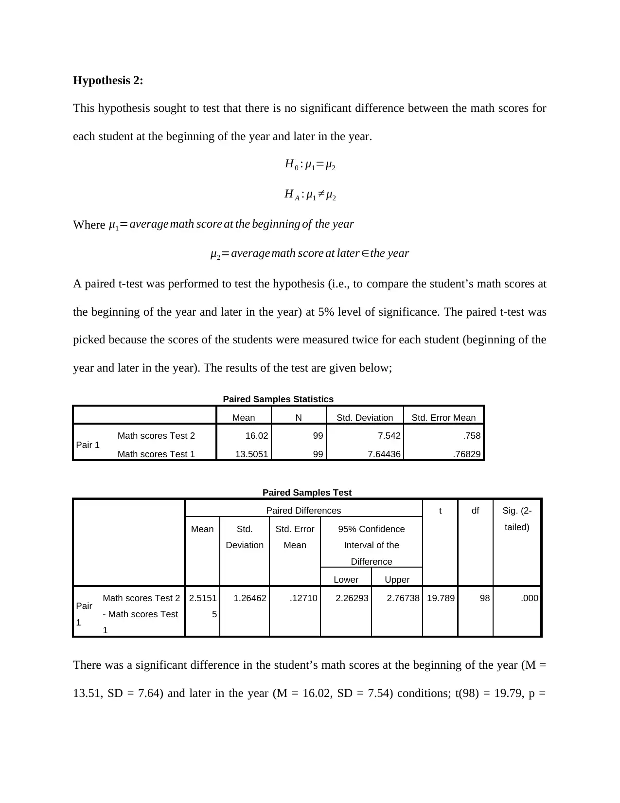
There was a significant difference in the student’s math scores at the beginning of the year (M =
13.51, SD = 7.64) and later in the year (M = 16.02, SD = 7.54) conditions; t(98) = 19.79, p =
This hypothesis sought to test that there is no significant difference between the math scores for
each student at the beginning of the year and later in the year.
H0 : μ1=μ2
H A : μ1 ≠ μ2
Where μ1=average math score at the beginning of the year
μ2=average math score at later ∈the year
A paired t-test was performed to test the hypothesis (i.e., to compare the student’s math scores at
the beginning of the year and later in the year) at 5% level of significance. The paired t-test was
picked because the scores of the students were measured twice for each student (beginning of the
year and later in the year). The results of the test are given below;
Paired Samples Statistics
Mean N Std. Deviation Std. Error Mean
Pair 1 Math scores Test 2 16.02 99 7.542 .758
Math scores Test 1 13.5051 99 7.64436 .76829
Paired Samples Test
Paired Differences t df Sig. (2-
tailed)Mean Std.
Deviation
Std. Error
Mean
95% Confidence
Interval of the
Difference
Lower Upper
Pair
1
Math scores Test 2
- Math scores Test
1
2.5151
5
1.26462 .12710 2.26293 2.76738 19.789 98 .000
There was a significant difference in the student’s math scores at the beginning of the year (M =
13.51, SD = 7.64) and later in the year (M = 16.02, SD = 7.54) conditions; t(98) = 19.79, p =
⊘ This is a preview!⊘
Do you want full access?
Subscribe today to unlock all pages.
Trusted by 1+ million students worldwide
0.000. These results suggest that students did improve in their math scores since they on overage
had higher scores later in the year as compared to the beginning of the year.
Hypothesis 3:
This hypothesis sought to test that there is no significant difference between the science scores
for each student at the beginning of the year and later in the year.
H0 : μ1=μ2
H A : μ1 ≠ μ2
Where μ1=average science score at the beginning of the year
μ2=average science score at later ∈the year
A paired t-test was performed to test the hypothesis (i.e., to compare the student’s science scores
at the beginning of the year and later in the year) at 5% level of significance. The paired t-test
was picked because the scores of the students were measured twice for each student (beginning
of the year and later in the year). The results of the test are given below;
Paired Samples Statistics
Mean N Std. Deviation Std. Error Mean
Pair 1 Science scores Test 2 19.02 99 7.542 .758
Science scores Test 1 16.0000 99 7.70502 .77438
Paired Samples Test
Paired Differences t df Sig. (2-
tailed)Mean Std.
Deviation
Std. Error
Mean
95% Confidence
Interval of the
Difference
Lower Upper
Pair 1
Science scores Test
2 - Science scores
Test 1
3.02020 1.07836 .10838 2.80513 3.23528 27.867 98 .000
Paraphrase This Document
Need a fresh take? Get an instant paraphrase of this document with our AI Paraphraser
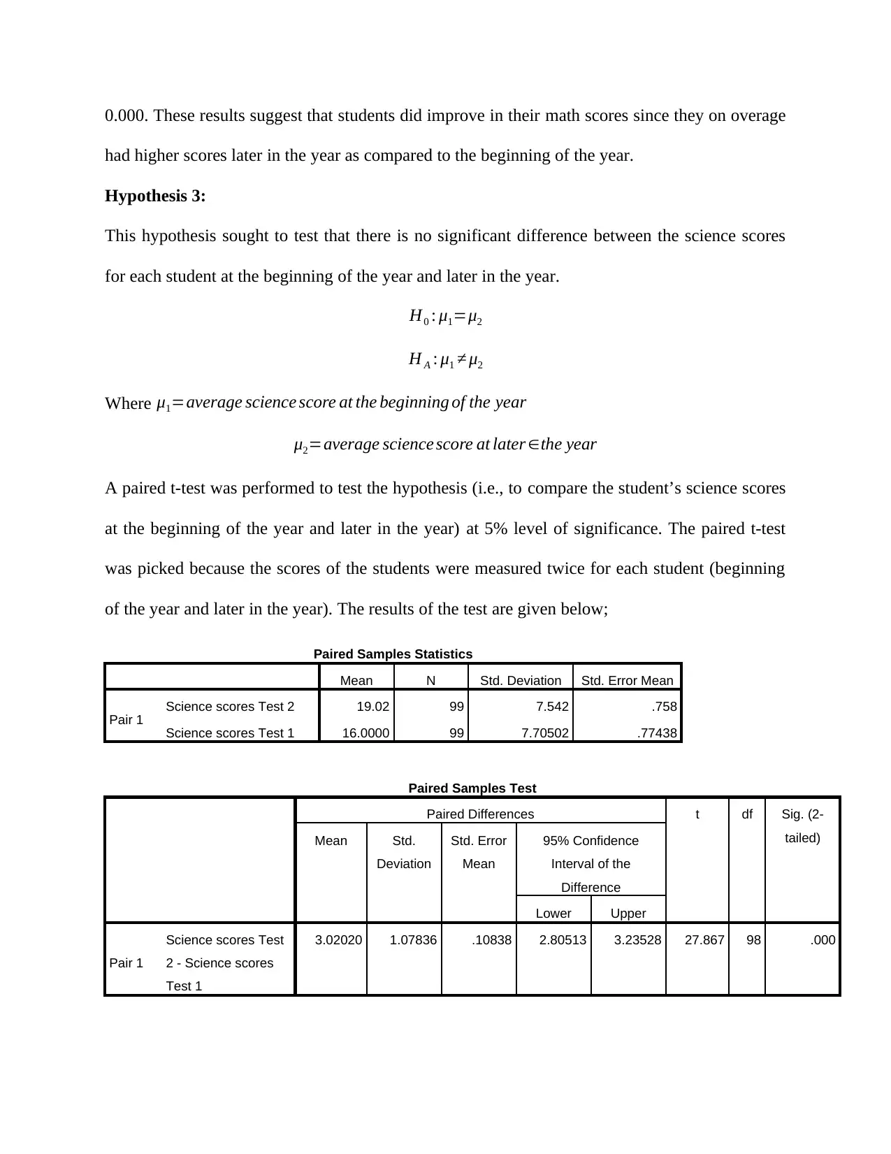
There was a significant difference in the student’s science scores at the beginning of the year (M
= 16.00, SD = 7.71) and later in the year (M = 19.02, SD = 7.54) conditions; t(98) = 27.87, p =
0.000. These results suggest that students did improve in their science scores since they on
overage had higher scores later in the year as compared to the beginning of the year.
Question 3: Do gender differences exist in math, science, and reading scores?
For this question, we sought to test three different hypotheses. The hypotheses are given as
follows;
Hypothesis 1:
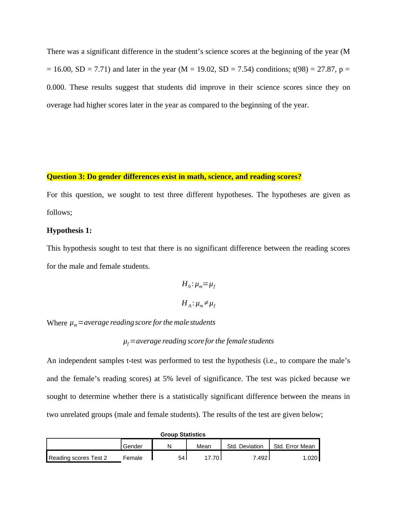
This hypothesis sought to test that there is no significant difference between the reading scores
for the male and female students.
H0 : μm=μf
H A : μm ≠ μf
Where μm =average reading score for the male students
μf =average reading score for the female students
An independent samples t-test was performed to test the hypothesis (i.e., to compare the male’s
and the female’s reading scores) at 5% level of significance. The test was picked because we
sought to determine whether there is a statistically significant difference between the means in
two unrelated groups (male and female students). The results of the test are given below;
Group Statistics
Gender N Mean Std. Deviation Std. Error Mean
Reading scores Test 2 Female 54 17.70 7.492 1.020
= 16.00, SD = 7.71) and later in the year (M = 19.02, SD = 7.54) conditions; t(98) = 27.87, p =
0.000. These results suggest that students did improve in their science scores since they on
overage had higher scores later in the year as compared to the beginning of the year.
Question 3: Do gender differences exist in math, science, and reading scores?
For this question, we sought to test three different hypotheses. The hypotheses are given as
follows;
Hypothesis 1:
This hypothesis sought to test that there is no significant difference between the reading scores
for the male and female students.
H0 : μm=μf
H A : μm ≠ μf
Where μm =average reading score for the male students
μf =average reading score for the female students
An independent samples t-test was performed to test the hypothesis (i.e., to compare the male’s
and the female’s reading scores) at 5% level of significance. The test was picked because we
sought to determine whether there is a statistically significant difference between the means in
two unrelated groups (male and female students). The results of the test are given below;
Group Statistics
Gender N Mean Std. Deviation Std. Error Mean
Reading scores Test 2 Female 54 17.70 7.492 1.020
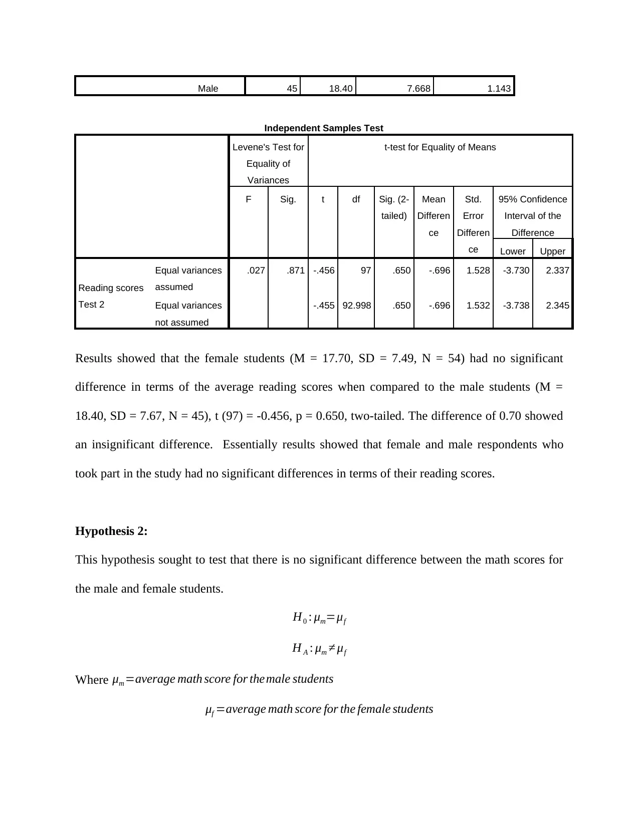
Male 45 18.40 7.668 1.143
Independent Samples Test
Levene's Test for
Equality of
Variances
t-test for Equality of Means
F Sig. t df Sig. (2-
tailed)
Mean
Differen
ce
Std.
Error
Differen
ce
95% Confidence
Interval of the
Difference
Lower Upper
Reading scores
Test 2
Equal variances
assumed
.027 .871 -.456 97 .650 -.696 1.528 -3.730 2.337
Equal variances
not assumed
-.455 92.998 .650 -.696 1.532 -3.738 2.345
Results showed that the female students (M = 17.70, SD = 7.49, N = 54) had no significant
difference in terms of the average reading scores when compared to the male students (M =
18.40, SD = 7.67, N = 45), t (97) = -0.456, p = 0.650, two-tailed. The difference of 0.70 showed
an insignificant difference. Essentially results showed that female and male respondents who
took part in the study had no significant differences in terms of their reading scores.
Hypothesis 2:
This hypothesis sought to test that there is no significant difference between the math scores for
the male and female students.
H0 : μm=μf
H A : μm ≠ μf
Where μm =average math score for themale students
μf =average math score for the female students
⊘ This is a preview!⊘
Do you want full access?
Subscribe today to unlock all pages.
Trusted by 1+ million students worldwide
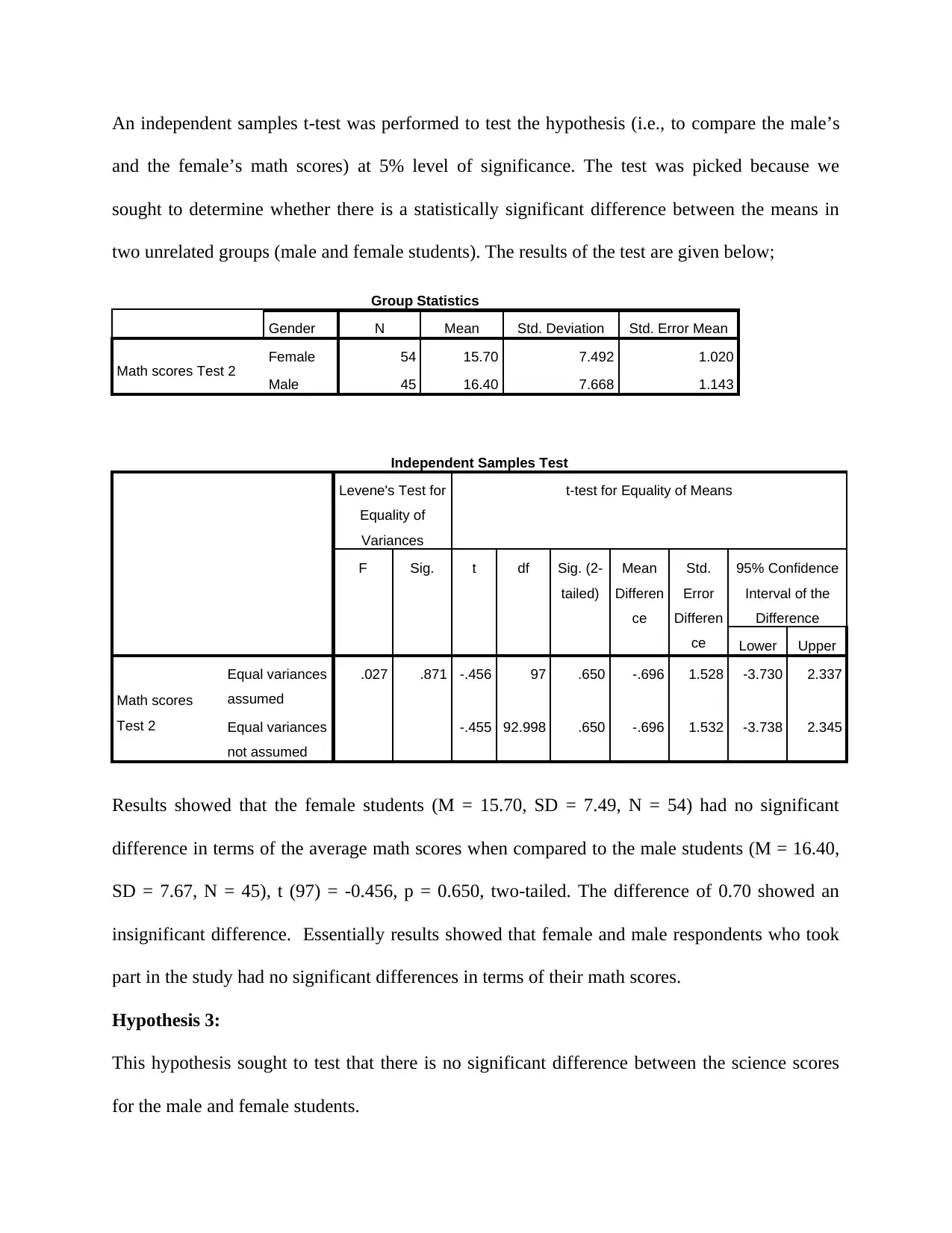
An independent samples t-test was performed to test the hypothesis (i.e., to compare the male’s
and the female’s math scores) at 5% level of significance. The test was picked because we
sought to determine whether there is a statistically significant difference between the means in
two unrelated groups (male and female students). The results of the test are given below;
Group Statistics
Gender N Mean Std. Deviation Std. Error Mean
Math scores Test 2 Female 54 15.70 7.492 1.020
Male 45 16.40 7.668 1.143
Independent Samples Test
Levene's Test for
Equality of
Variances
t-test for Equality of Means
F Sig. t df Sig. (2-
tailed)
Mean
Differen
ce
Std.
Error
Differen
ce
95% Confidence
Interval of the
Difference
Lower Upper
Math scores
Test 2
Equal variances
assumed
.027 .871 -.456 97 .650 -.696 1.528 -3.730 2.337
Equal variances
not assumed
-.455 92.998 .650 -.696 1.532 -3.738 2.345
Results showed that the female students (M = 15.70, SD = 7.49, N = 54) had no significant
difference in terms of the average math scores when compared to the male students (M = 16.40,
SD = 7.67, N = 45), t (97) = -0.456, p = 0.650, two-tailed. The difference of 0.70 showed an
insignificant difference. Essentially results showed that female and male respondents who took
part in the study had no significant differences in terms of their math scores.
Hypothesis 3:
This hypothesis sought to test that there is no significant difference between the science scores
for the male and female students.
Paraphrase This Document
Need a fresh take? Get an instant paraphrase of this document with our AI Paraphraser
H0 : μm=μf
H A : μm ≠ μf
Where μm =average science score for the male students
μf =average science score for the female students
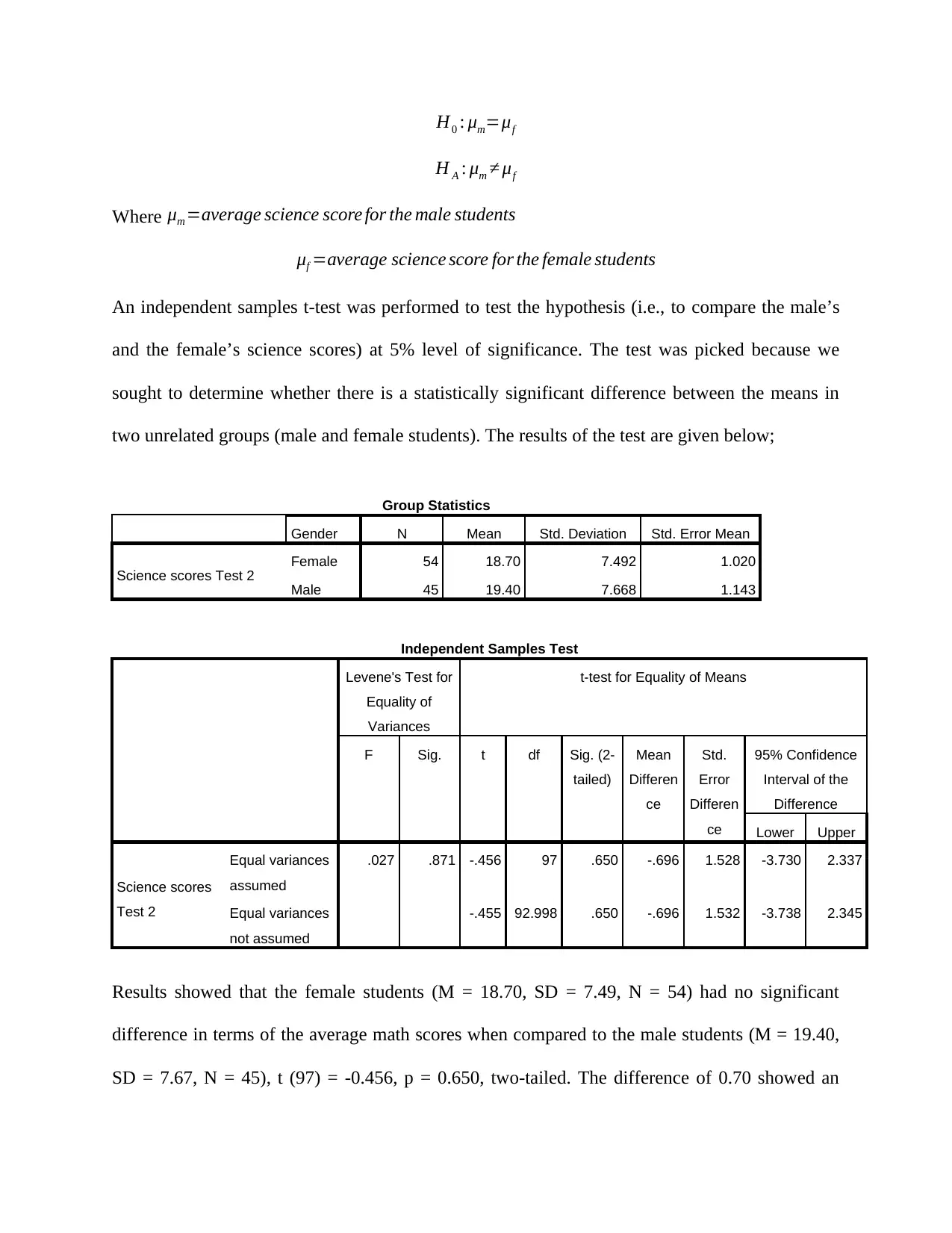
An independent samples t-test was performed to test the hypothesis (i.e., to compare the male’s
and the female’s science scores) at 5% level of significance. The test was picked because we
sought to determine whether there is a statistically significant difference between the means in
two unrelated groups (male and female students). The results of the test are given below;
Group Statistics
Gender N Mean Std. Deviation Std. Error Mean
Science scores Test 2 Female 54 18.70 7.492 1.020
Male 45 19.40 7.668 1.143
Independent Samples Test
Levene's Test for
Equality of
Variances
t-test for Equality of Means
F Sig. t df Sig. (2-
tailed)
Mean
Differen
ce
Std.
Error
Differen
ce
95% Confidence
Interval of the
Difference
Lower Upper
Science scores
Test 2
Equal variances
assumed
.027 .871 -.456 97 .650 -.696 1.528 -3.730 2.337
Equal variances
not assumed
-.455 92.998 .650 -.696 1.532 -3.738 2.345
Results showed that the female students (M = 18.70, SD = 7.49, N = 54) had no significant
difference in terms of the average math scores when compared to the male students (M = 19.40,
SD = 7.67, N = 45), t (97) = -0.456, p = 0.650, two-tailed. The difference of 0.70 showed an
H A : μm ≠ μf
Where μm =average science score for the male students
μf =average science score for the female students
An independent samples t-test was performed to test the hypothesis (i.e., to compare the male’s
and the female’s science scores) at 5% level of significance. The test was picked because we
sought to determine whether there is a statistically significant difference between the means in
two unrelated groups (male and female students). The results of the test are given below;
Group Statistics
Gender N Mean Std. Deviation Std. Error Mean
Science scores Test 2 Female 54 18.70 7.492 1.020
Male 45 19.40 7.668 1.143
Independent Samples Test
Levene's Test for
Equality of
Variances
t-test for Equality of Means
F Sig. t df Sig. (2-
tailed)
Mean
Differen
ce
Std.
Error
Differen
ce
95% Confidence
Interval of the
Difference
Lower Upper
Science scores
Test 2
Equal variances
assumed
.027 .871 -.456 97 .650 -.696 1.528 -3.730 2.337
Equal variances
not assumed
-.455 92.998 .650 -.696 1.532 -3.738 2.345
Results showed that the female students (M = 18.70, SD = 7.49, N = 54) had no significant
difference in terms of the average math scores when compared to the male students (M = 19.40,
SD = 7.67, N = 45), t (97) = -0.456, p = 0.650, two-tailed. The difference of 0.70 showed an
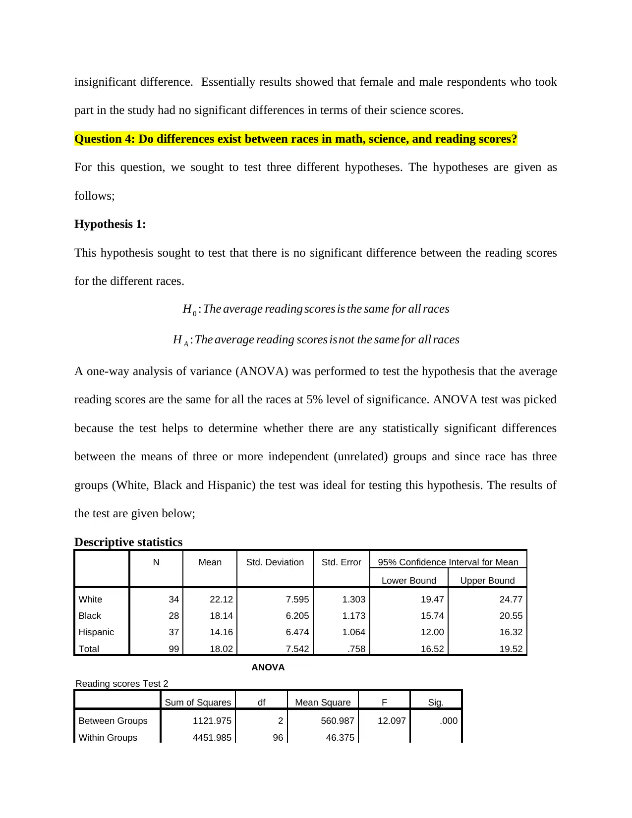
insignificant difference. Essentially results showed that female and male respondents who took
part in the study had no significant differences in terms of their science scores.
Question 4: Do differences exist between races in math, science, and reading scores?
For this question, we sought to test three different hypotheses. The hypotheses are given as
follows;
Hypothesis 1:
This hypothesis sought to test that there is no significant difference between the reading scores
for the different races.
H0 :The average reading scores is the same for all races
H A :The average reading scores isnot the same for all races
A one-way analysis of variance (ANOVA) was performed to test the hypothesis that the average
reading scores are the same for all the races at 5% level of significance. ANOVA test was picked
because the test helps to determine whether there are any statistically significant differences
between the means of three or more independent (unrelated) groups and since race has three
groups (White, Black and Hispanic) the test was ideal for testing this hypothesis. The results of
the test are given below;
Descriptive statistics
N Mean Std. Deviation Std. Error 95% Confidence Interval for Mean
Lower Bound Upper Bound
White 34 22.12 7.595 1.303 19.47 24.77
Black 28 18.14 6.205 1.173 15.74 20.55
Hispanic 37 14.16 6.474 1.064 12.00 16.32
Total 99 18.02 7.542 .758 16.52 19.52
ANOVA
Reading scores Test 2
Sum of Squares df Mean Square F Sig.
Between Groups 1121.975 2 560.987 12.097 .000
Within Groups 4451.985 96 46.375
⊘ This is a preview!⊘
Do you want full access?
Subscribe today to unlock all pages.
Trusted by 1+ million students worldwide
1 out of 42


Your All-in-One AI-Powered Toolkit for Academic Success.
+13062052269
info@desklib.com
Available 24*7 on WhatsApp / Email
![[object Object]](/_next/static/media/star-bottom.7253800d.svg)
Unlock your academic potential
Copyright © 2020–2026 A2Z Services. All Rights Reserved. Developed and managed by ZUCOL.