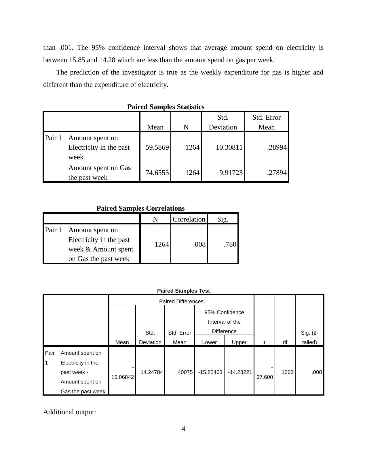
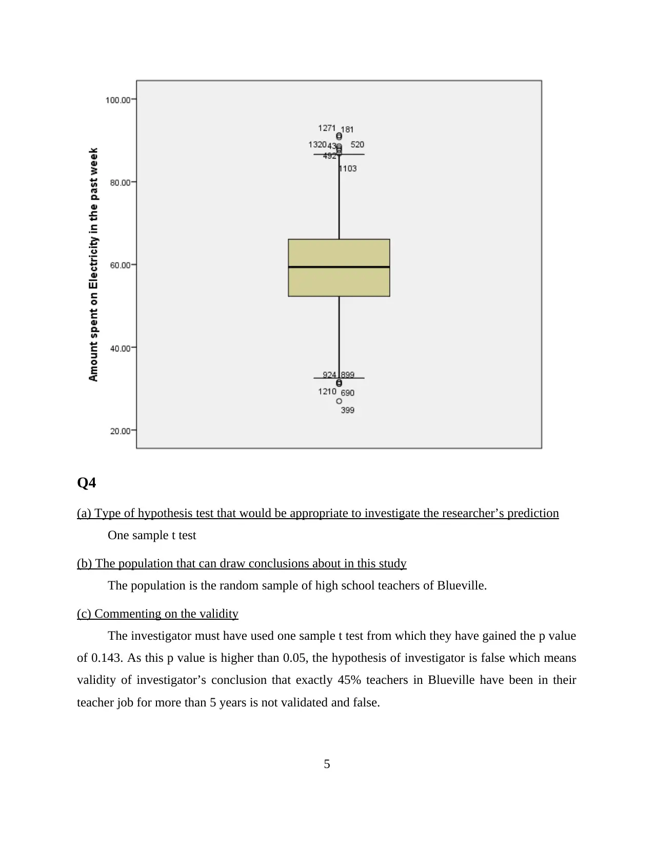
Statistics Assignment: Analysis of Californian Adults using T-tests

This document presents a solved statistics assignment focusing on t-tests. The assignment analyzes data related to Californian adults, covering one-sample, independent samples, and paired samples t-tests. The solution includes the analysis of time spent on leisure walks, hours worked by different age groups, and expenditure on gas and electricity. The results are interpreted, and conclusions are drawn based on the t-test results, including p-values and confidence intervals. The assignment also addresses the type of hypothesis test appropriate for a given prediction and comments on the validity of the conclusions. The data analysis is performed using statistical software, and the findings are presented with supporting statistical output.

Statistics

Contents
Q1 - One-sample t-test [Time walked for leisure]...........................................................................1
Q2 - Independent samples t-test [Hours worked / Age Group].......................................................1
Q3 - Paired samples t- test [Electricity / Gas].................................................................................3
Q4....................................................................................................................................................5
(a) Type of hypothesis test that would be appropriate to investigate the researcher’s prediction
.....................................................................................................................................................5
(b) The population that can draw conclusions about in this study..............................................5
(c) Commenting on the validity...................................................................................................5

Q1 - One-sample t-test [Time walked for leisure]
A study was conducted which indicated the time Californian adults spent on walking for
Leisure is 35 minutes per week on an average. In order to identify whether this walking time has
changed or not a random sample of 1500 people is taken.
From the one sample t test results attached below, it has been seen that average Leisure walk
per week of the 1500 Californian adults is 34.36 minutes. This average of 34.36 is too close to
the time identified in previous investigation which was 35 minutes. The results of one sample t
test also shows that the mean difference of time walked for Leisure is significant t(951) = 28.45,
p = .000. The confidence interval shows the average weekly walk for Leisure is between 31.99
minutes and 36.73 minutes.
So, the weekly Leisure Walk of Californian adults have slightly lowered down.
One-Sample Statistics
N Mean
Std.
Deviation
Std. Error
Mean
Time walked for leisure
[mins in previous week] 952 34.36 37.264 1.208
One-Sample Test
Test Value = 0
t df
Sig. (2-
tailed)
Mean
Difference
95% Confidence Interval
of the Difference
Lower Upper
Time walked for
leisure [mins in
previous week]
28.452 951 .000 34.362 31.99 36.73
Q2 - Independent samples t-test [Hours worked / Age Group]
An economist has predicted that Californian adults who are aged less than 40 years works
less hours than those who are 40 or old per week. In order to check this prediction, a sample
random of 1500 Californian adults has been taken from the entire data population of 6259. This
sample data is used to conduct independent samples t test.
1

From the results of the test conducted, it has been observed that the mean number of hours
worked per week by Californian adults aged less than 40 (M = 24.66, s =18.33, n =326) was
higher than the average working hours of Californian adults aged 40 or more (M = 14.71, s =
18.78, n = 1174). Also, the results shows that the difference between mean working hours is
significant, t(1498) = 8.506, p = .000. The confidence interval of independent samples t test
shows that people aged less than 40, works between 7.65 to 12.2 hours per week people aged 40
or more works between 7.68 to 12.22 hours per week.
As the significance of this test is significant then it can be said that prediction made by the
investigator is true at a certain level that Californian adults who are aged less than 40 years
works less hours than those who are 40 or old per week.
Group Statistics
Age Group N Mean
Std.
Deviation
Std. Error
Mean
Hours worked
[previous week]
Less than 40
years 326 24.66 18.338 1.016
40 years or older 1174 14.71 18.787 .548
Independent Samples Test
Levene's
Test for
Equality of
Variances t-test for Equality of Means
F Sig. t df
Sig.
(2-
tailed)
Mean
Difference
Std. Error
Difference
95%
Confidence
Interval of the
Difference
Lower Upper
Hours
worked
Equal
variances
assumed
3.800 .051 8.506 1498 .000 9.952 1.170 7.657 12.247
2

[previous
week]
Equal
variances
not
assumed
8.623 529.581 .000 9.952 1.154 7.685 12.220
Additional output:
Q3 - Paired samples t- test [Electricity / Gas]
A research believes that the amount spent on gas and electricity for Californian adults is
different. In order to check this prediction, the paired samples t test is conducted.
The results of the conducted test indicates that on an average, the expenditure done on gas
(M = 74.65, s = 9.91) was higher than the expenditure done on electricity (M = 59.58, s = 10.30).
This test also shows that the difference in the mean between amount spend for gas and electricity
spend in a week is (MD = 15.06, SD = 14.24) is significant t(1263) = 37.6, p = .000 which is less
3

than .001. The 95% confidence interval shows that average amount spend on electricity is
between 15.85 and 14.28 which are less than the amount spend on gas per week.
The prediction of the investigator is true as the weekly expenditure for gas is higher and
different than the expenditure of electricity.
Paired Samples Statistics
Mean N
Std.
Deviation
Std. Error
Mean
Pair 1 Amount spent on
Electricity in the past
week
59.5869 1264 10.30811 .28994
Amount spent on Gas
the past week 74.6553 1264 9.91723 .27894
Paired Samples Correlations
N Correlation Sig.
Pair 1 Amount spent on
Electricity in the past
week & Amount spent
on Gas the past week
1264 .008 .780
Paired Samples Test
Paired Differences
t df
Sig. (2-
tailed)Mean
Std.
Deviation
Std. Error
Mean
95% Confidence
Interval of the
Difference
Lower Upper
Pair
1
Amount spent on
Electricity in the
past week -
Amount spent on
Gas the past week
-
15.06842 14.24784 .40075 -15.85463 -14.28221 -
37.600 1263 .000
Additional output:
4

Q4
(a) Type of hypothesis test that would be appropriate to investigate the researcher’s prediction
One sample t test
(b) The population that can draw conclusions about in this study
The population is the random sample of high school teachers of Blueville.
(c) Commenting on the validity
The investigator must have used one sample t test from which they have gained the p value
of 0.143. As this p value is higher than 0.05, the hypothesis of investigator is false which means
validity of investigator’s conclusion that exactly 45% teachers in Blueville have been in their
teacher job for more than 5 years is not validated and false.
5