Solved STA101 Statistics for Business Assignment 1: Detailed Analysis
VerifiedAdded on 2023/06/04
|13
|1672
|354
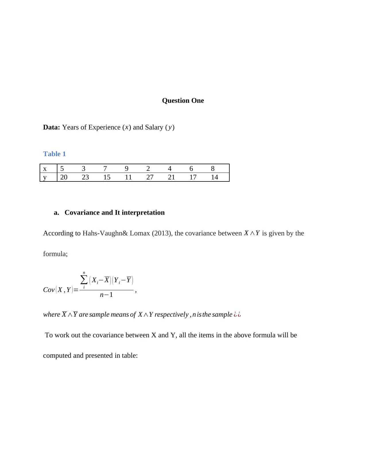
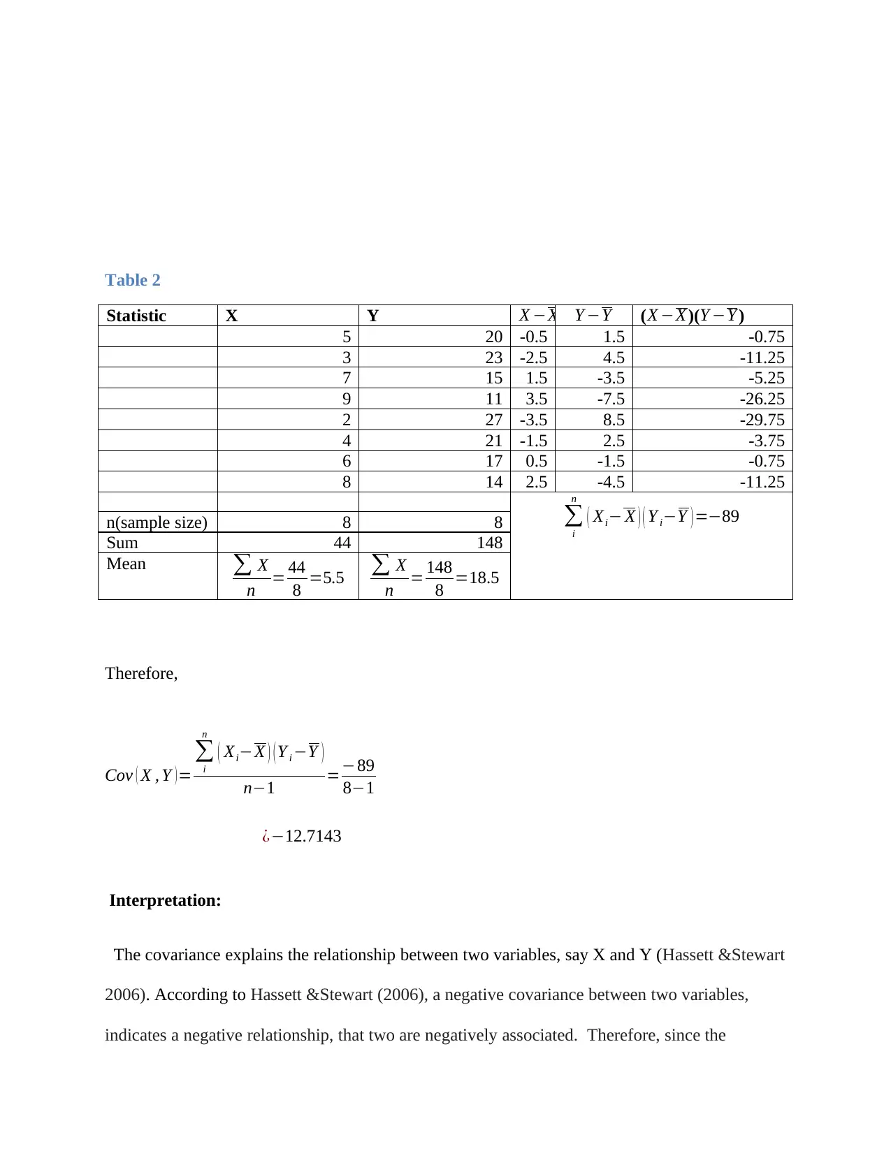
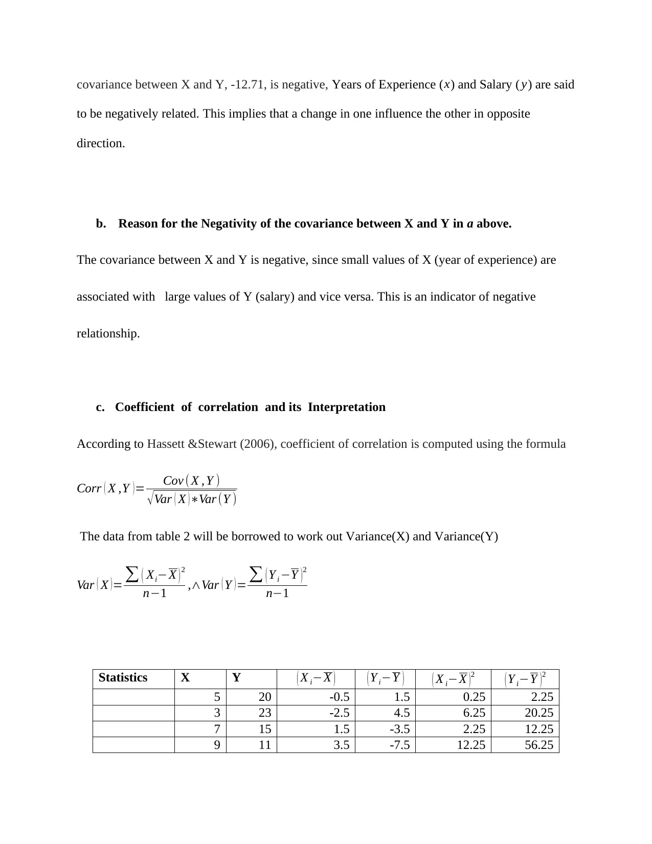
Homework Assignment
AI Summary
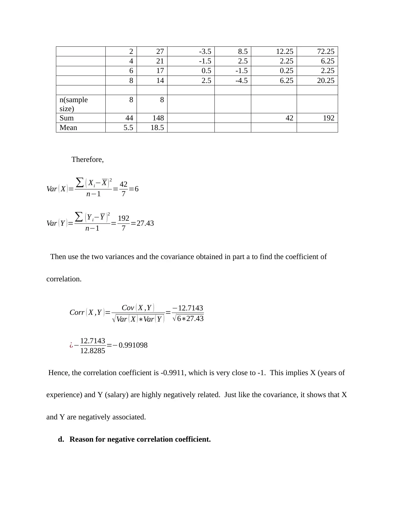
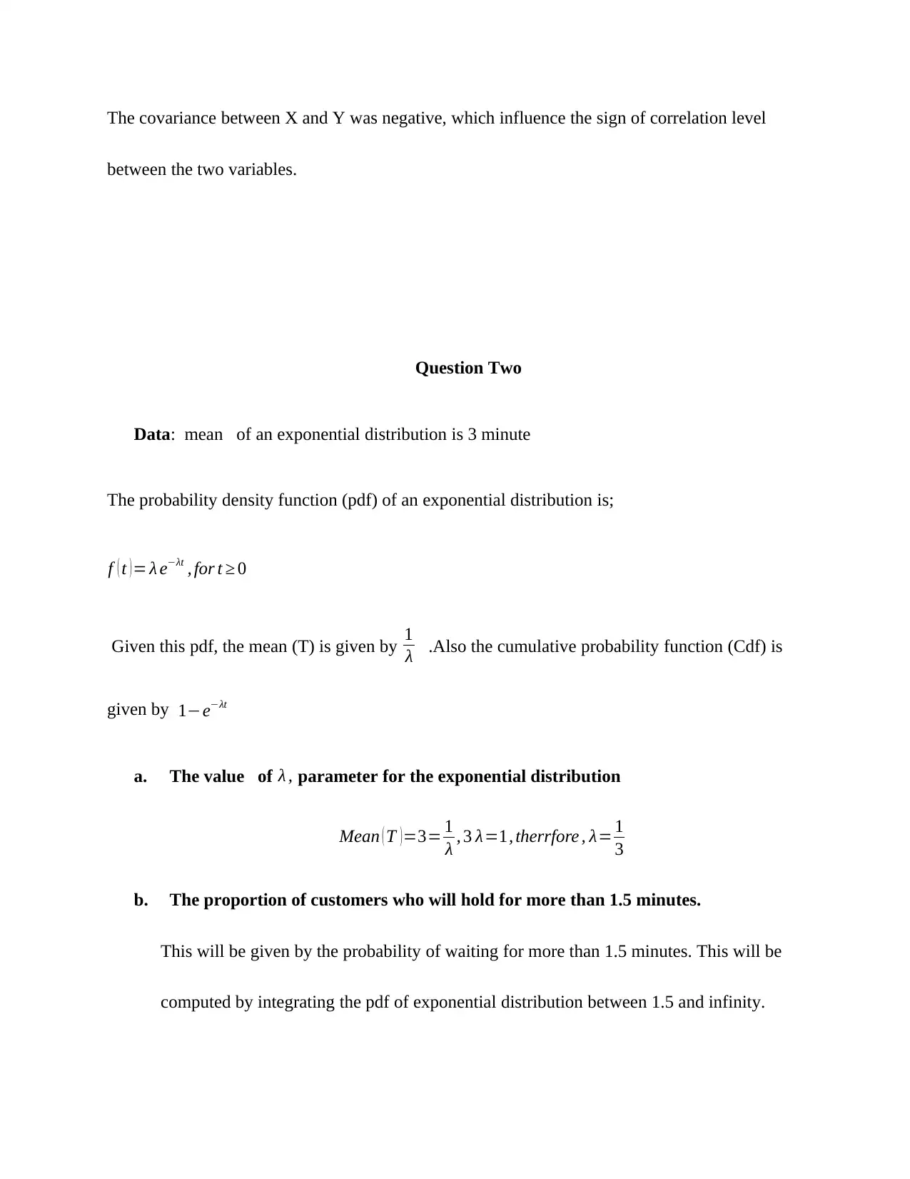
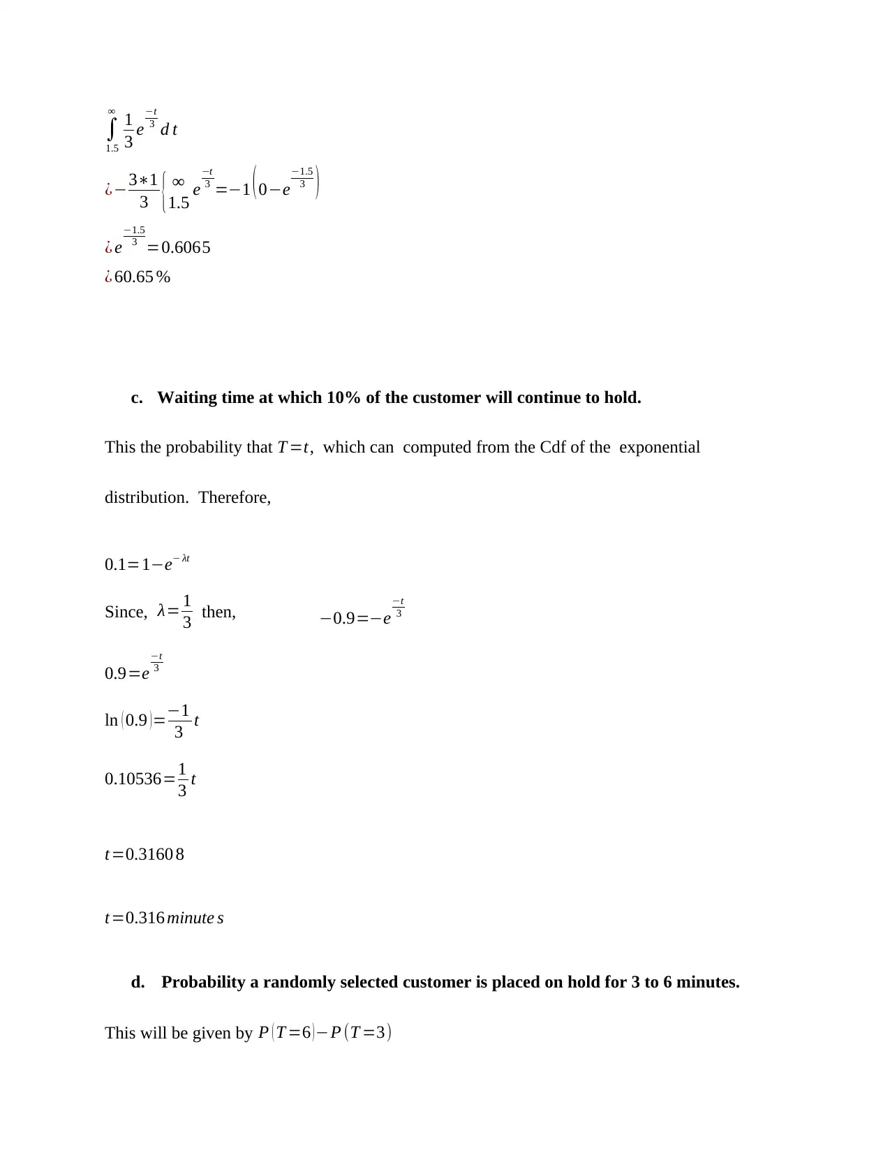
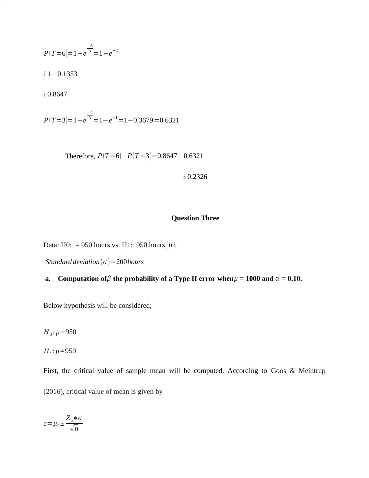
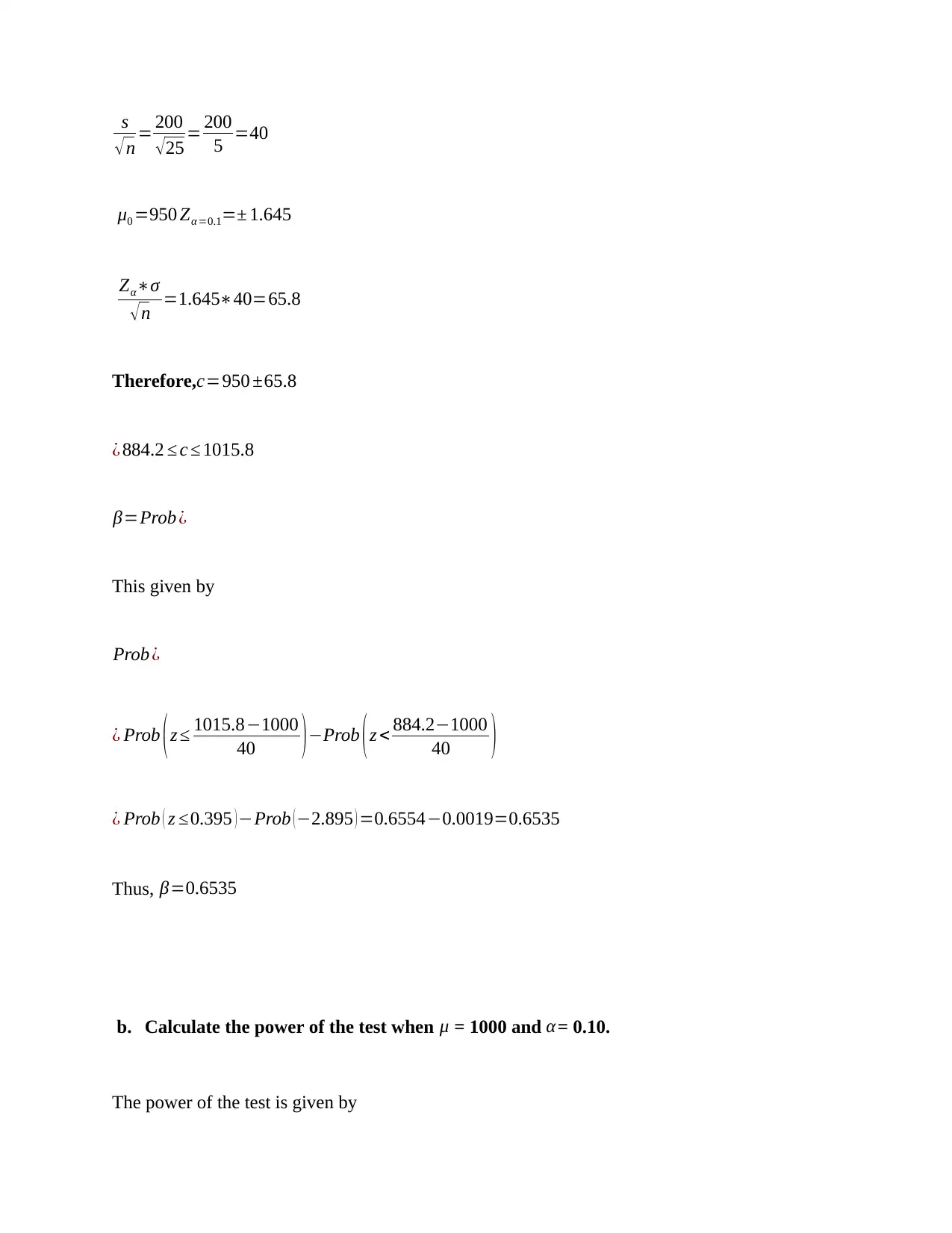
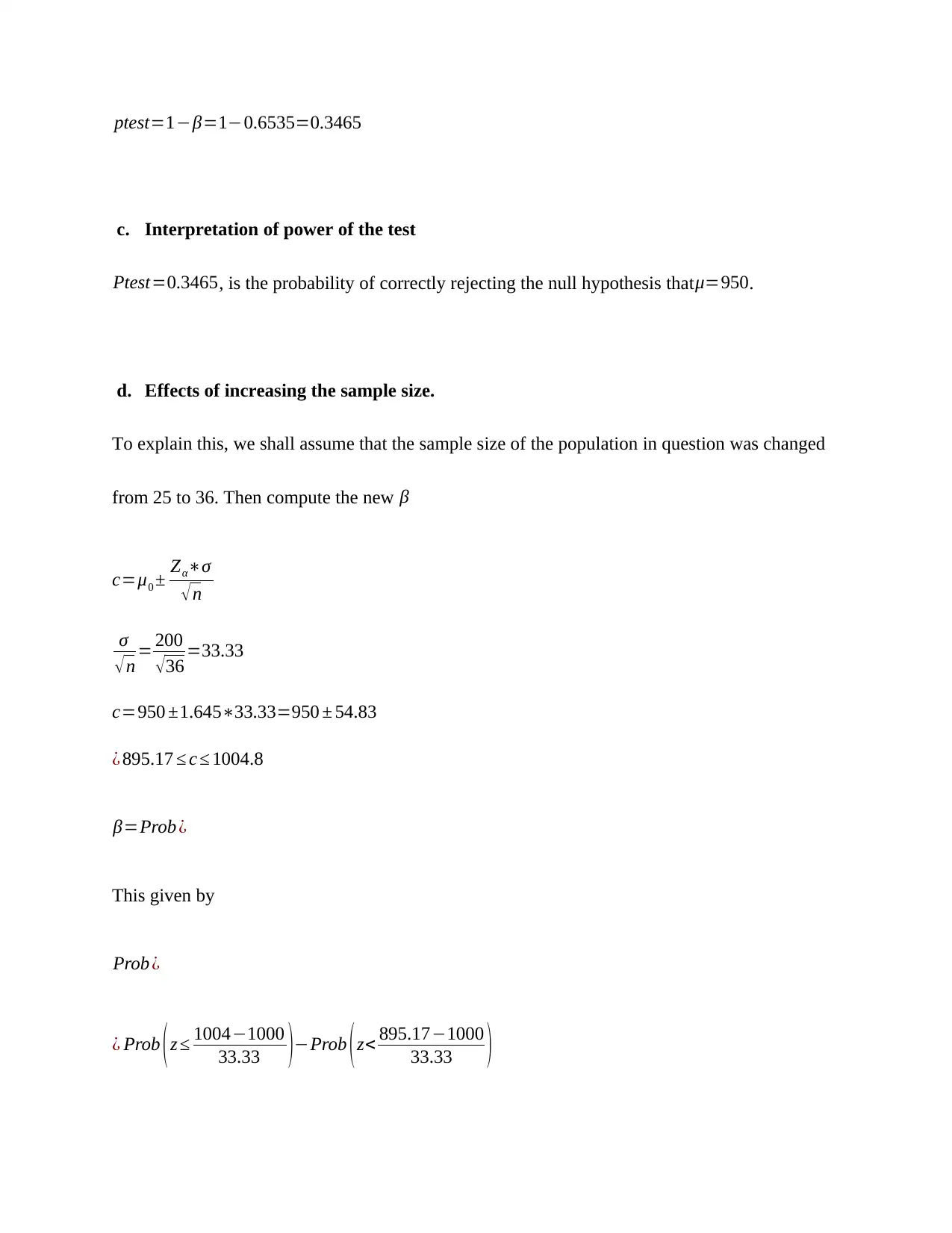
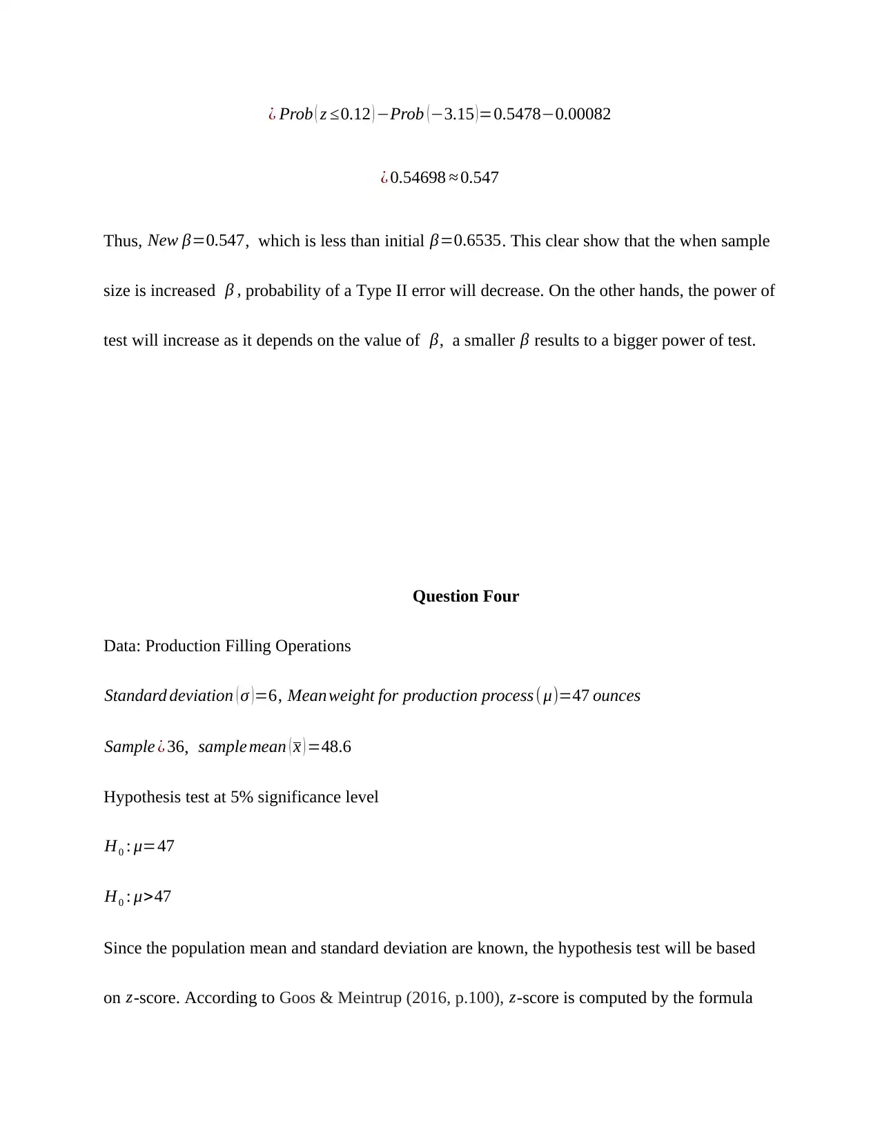
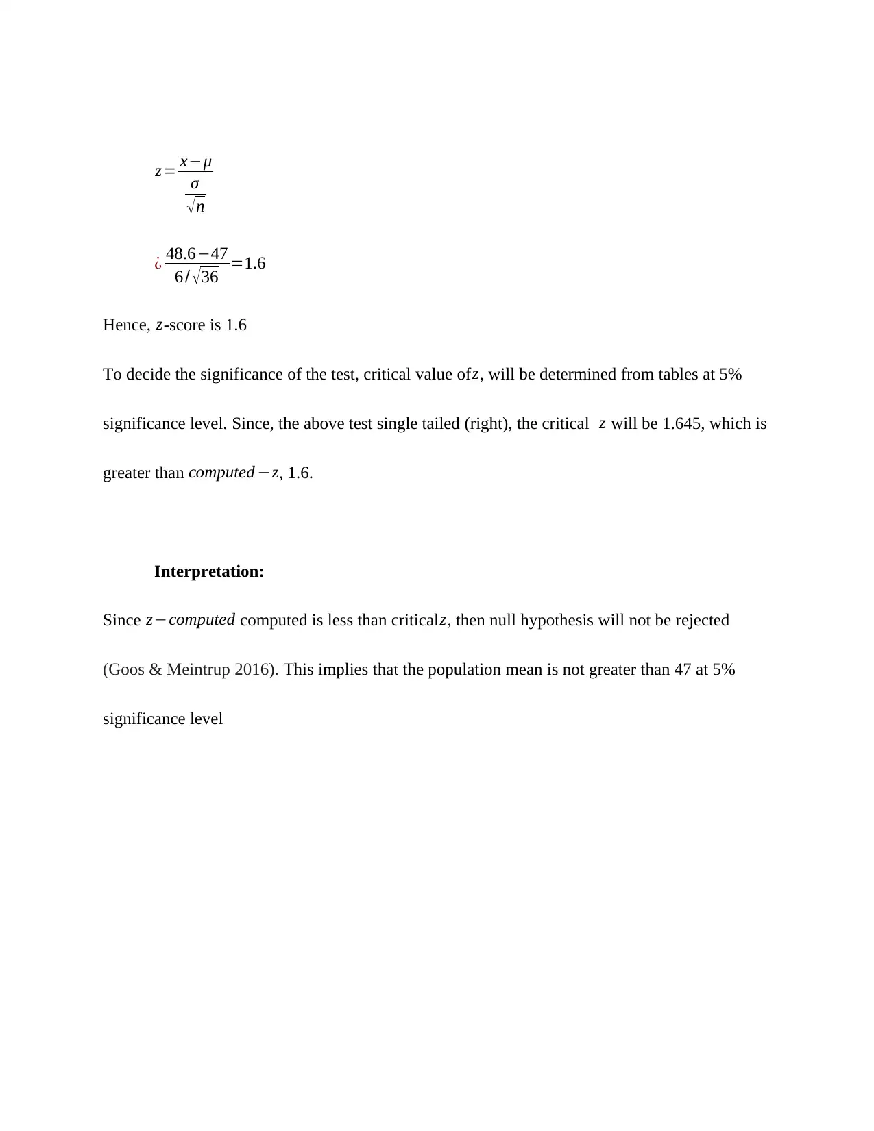
This assignment solution covers key statistical concepts within a business context. It includes the calculation and interpretation of covariance and correlation between years of experience and salary, providing reasons for negative relationships. The solution also addresses problems related to exponential distribution, calculating probabilities and waiting times. Furthermore, it includes hypothesis testing, computation of Type II error probability, power of the test, and the effects of changing sample size. A final question focuses on hypothesis testing for production filling operations, using z-scores to determine the significance of the test. Desklib provides this document, along with numerous other solved assignments and study resources, to aid students in their academic pursuits.
1 out of 13
Related Documents


Your All-in-One AI-Powered Toolkit for Academic Success.
+13062052269
info@desklib.com
Available 24*7 on WhatsApp / Email
![[object Object]](/_next/static/media/star-bottom.7253800d.svg)
Copyright © 2020–2026 A2Z Services. All Rights Reserved. Developed and managed by ZUCOL.