STA2300 Data Analysis S3, 18 Assignment 3 Solutions - Statistics

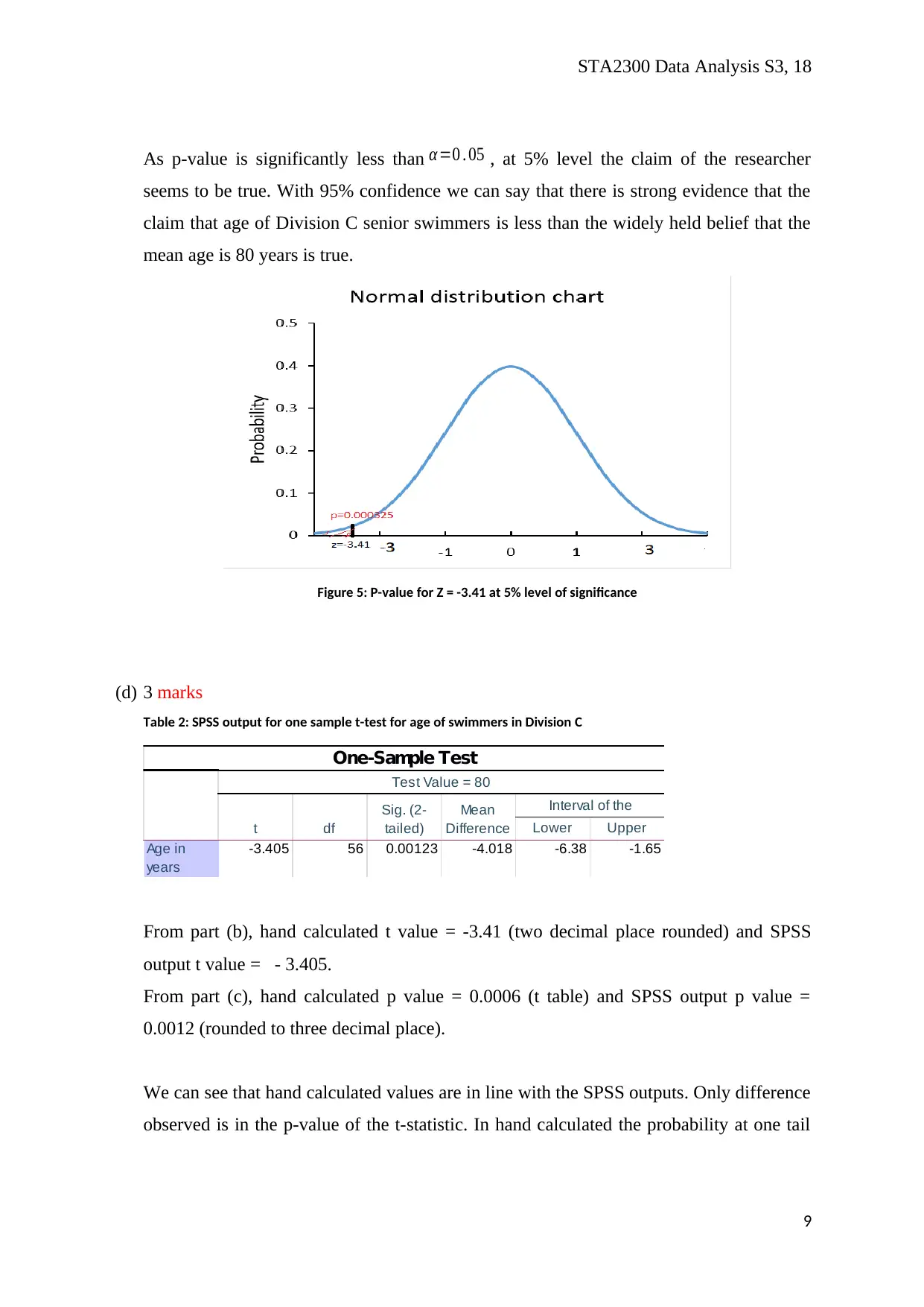
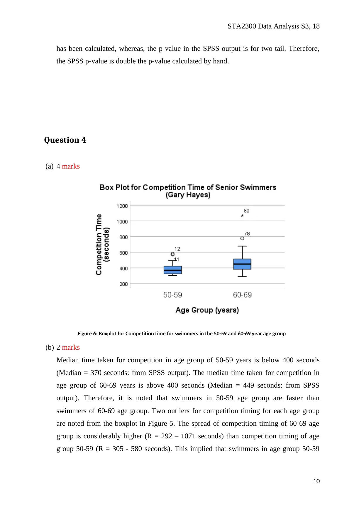
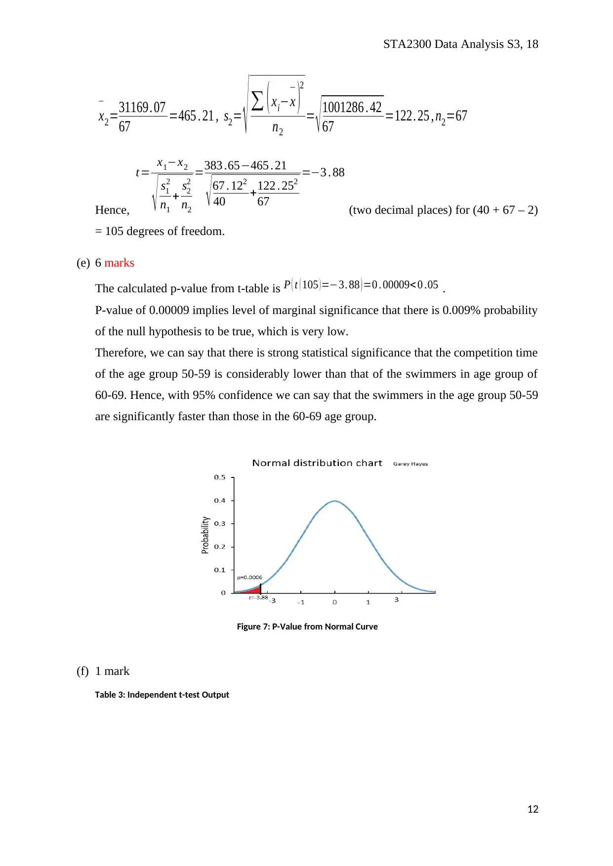
This document contains the solutions for Assignment 3 of the STA2300 Data Analysis course. The assignment focuses on statistical analysis, covering topics such as hypothesis testing, confidence intervals, and t-tests. The solution begins by analyzing the proportion of swimmers in Division A, performing a one-sample test of proportions, and discussing the assumptions and calculations involved. It then proceeds to construct confidence intervals for the mean age of swimmers in Division C, including the assumptions and SPSS output. Furthermore, the solution includes a one-sample t-test to assess the claim about the average age of senior swimmers in Division C. Finally, the assignment compares the competition times of swimmers in different age groups using boxplots, independent t-tests, and discusses the relevant assumptions and statistical outcomes. The solutions provide detailed explanations, calculations, and interpretations of the statistical findings, including p-values and confidence levels.

STA2300 Data Analysis S3, 18
Assignment 3 Solutions
Due Date: 29 January, 2019
1

STA2300 Data Analysis S3, 18
Question 1
(a) 2 marks
Variable of interest: Number of swimmers (X) in Division A or the fastest division is
the variable of interest. We assume here that qualifying times for division A for each
swimmer is independent of others and have probability of (0.2) to qualify for the
aforesaid division.
Sample Statistic: Amongst 186 total swimmers, 43 swimmers (23.1%) are in Division
A, 86 swimmers (46.2%) are in Division B, and 57 (30.6%) swimmers are in Division C.
Mean and Median for the division of the swimmers was Division B.
Figure 1: Percentage distribution of Swimmers in Divisions
(b) 3 marks
Hypotheses: Null hypothesis: H0: (p = 0.2) and the right tail Alternate hypothesis is HA:
( p>0 .2 )
Here, p denotes the probability that number of swimmers in Division A is 20% or 0.2.
The alternate hypothesis is in accordance with the researchers claim that number of
swimmers in Division A is more than 20%.
(c) 4 marks
Assumptions: The assumptions for one sample test of proportions are guided by
Binomial Model X ~ B ( n , p ) , where n = 186 is the number of swimmers and p = 0.2 is the
proportion or percentage f swimmers in Division A. Here the sample size was
considerably large ( n≥30 ) and therefore we will use normal approximation to binomial
model, by Central Limit Theorem (CLT).
2

STA2300 Data Analysis S3, 18
Rule of Sample Proportions:
According to the said rule for sample proportions, np≥10 and n ( 1− p ) ≥10 should be
satisfied for the sampling distribution to be normally distributed.
Here, np=186∗0. 2=37. 2>10 and n ( 1− p ) =186∗0 . 8=148. 8>10 . Rule of sample
proportion is satisfied and the sampling distribution will have SE (standard error) of
√ p ( 1− p )
n = √ 0. 2∗0 .8
186 =0. 03 .
(d) 2 marks
The test statistic for one sample test of proportion is
Z = p
^¿ − p
√ p ( 1− p )
n
¿
where p
^¿
¿ is sample
proportion and p
^¿=43
186 =0 .23
¿ ,
Z = 0 . 23−0. 2
√ 0. 2∗0 .8
186
=1 .023
(e) 6 marks
Considering level of significance, α =0 . 05 for this right tail test, and using the Z-table we
get p=P ( Z >1 . 023 ) =0 . 1532> 0 .05 . As the p value is greater than level of significance,
the null hypothesis cannot be rejected at 5% level.
Figure 2: P-Value plot in Normal Curve
3

STA2300 Data Analysis S3, 18
Therefore, we can conclude that there is not enough statistical evidence to support the
researcher’s belief that in recent year’s number of swimmers in Division A has grown
and surpassed the fastest 20% swimmers cut-off point. There is almost 15.32% chance
that fastest 20% swimmers are only in the Division A, and the probability is large enough
for not rejecting the null hypothesis.
(f) 4 marks
If Swimming Association wants to ensure that the margin error estimate of 99%
confidence is 0.02 of the actual proportion of senior swimmers in Group A, then the
minimum sample size is found as using a conservative method to determine sample size,
n= p
^¿∗¿ ¿
¿ ¿¿ Swimmers
(g) 3 marks
We get the required number of swimmers to ensure that the margin error estimate of 99%
confidence is 0.02 of the actual proportion of senior swimmers in Group A, using actual
proportion from the sample, then required sample size is,
n= p
^¿∗¿ ¿
¿ ¿¿ Swimmers
The impact of choosing the actual proportion from the sample is that number of
swimmers required will be considerable less, and this could result in less time and cost
for the research.
4

STA2300 Data Analysis S3, 18
Question 2
(a) 6 marks
Assumptions for Confidence Interval:
First, we assume that the swimmers are chosen randomly from the population of
swimmers. Secondly, number of the swimmers in Division-C are 57, which is greater
than 30. Hence, CLT can be applied on the distribution of the age of the swimmers to
establish that the data follows to a normal distribution. Third, it is also assumed that the
number of swimmers in Division-C is less than 10% of such swimmers in the population.
Assumptions for Hypothesis Testing:
The dependent variable, age of the swimmers in Division-C is continuous (interval/ratio).
The observations of age of the swimmers in Division-C are independent of one another.
The age of swimmers in Division-C, the dependent variable, is normally distributed. The
proof is accumulated from Shapiro-Wilk test for normality (W = 0.975, p = 0.275).
The age of swimmers in Division-C, the dependent variable does not contain any outliers.
The proof is the normal Q-Q plot and box plot of age for the swimmers in Division C.
Figure 3: Q-Q plot for age of the swimmers in division C
5

STA2300 Data Analysis S3, 18
Figure 4: Box plot for age of the swimmers in division C
(b) 6 marks
95% confidence interval:
Table 1: SPSS output for Descriptive Summary including 95% confidence interval
Statistic Std. Error
75.98 1.180
Lower
Bound
73.62
Upper
Bound
78.35
77.00
79.375
8.909
53
92
39
13
-0.497 0.316
-0.013 0.623
Maximum
Range
Interquartile Range
Skewness
Kurtosis
Descriptives
Age in
years
Mean
95% Confidence
Interval for Mean
Median
Variance
Std. Deviation
Minimum
The Confidence Interval for sample mean (
X
¿
) with unknown population standard
deviation is evaluated as,
X
¿
±Z∗ s
√ n
, where
X
¿
is the mean, Z is the chosen Z-value from
6

STA2300 Data Analysis S3, 18
the standard normal table, s is the sample standard deviation, and n is the number of
observations.
In this case,
X
¿
=75. 98
years, s = 8.91 years, n = 57 swimmers.
At 95%, the Z value = 1.96 (from Z-table).
So, the 95% confidence interval is calculated as,
75 .98±1 .96∗8 . 909
√ 57 =[ 75. 98±2. 37 ]=[ 73 .62 , 78. 35 ]
Hence, with 95% confidence, estimated population mean age for senior swimmers in
Division C in general is between 73.67 years and 78.35 years.
7

STA2300 Data Analysis S3, 18
Question 3
(a) 3 marks
For the one sample test for mean, the Null hypothesis: H0:
( μ=80 )
(Assumes that
average age of senior swimmers in Division C is 80)
And the left tail alternate hypothesis is HA:
( μ<80 )
(Assumes that average age of senior
swimmers in Division C in accordance to the researcher is less than 80), where
( μ )
is the
average age of senior swimmers in Division C.
(b) 2 marks
The sample size n = 57 is greater than 30, hence the sampling distribution of age of the
swimmers in Division C is considered to be normally distributed. The test statistic for
one sample test for mean is
t = x
¿
−μ
s / √ n with n-1 degrees of freedom. x
−
: The sample mean,
s: the sample standard deviation, and n is the sample size.
Average age of the swimmers in Division C is x
−
=75 . 98 years, standard deviation of age
in sample is s = 8.91 years, n = 57 swimmers in Division C.
Hence,
t= x
¿
−μ
s / √ n =75. 98−80
8. 91/ √ 57 =−4 . 02
1. 18 =−3 . 41 the value of the test statistic for one sample
test for mean
(c) 6 marks
Considering level of significance, α=0 . 05 for this right left test, and using the t-table we
get p=P ( t ( 56)<−3 . 41 ) =0 .0006 <0 .05 . As the p value is less than level of significance,
the null hypothesis can be rejected at 5% level.
8

STA2300 Data Analysis S3, 18
As p-value is significantly less than α=0 . 05 , at 5% level the claim of the researcher
seems to be true. With 95% confidence we can say that there is strong evidence that the
claim that age of Division C senior swimmers is less than the widely held belief that the
mean age is 80 years is true.
Figure 5: P-value for Z = -3.41 at 5% level of significance
(d) 3 marks
Table 2: SPSS output for one sample t-test for age of swimmers in Division C
Lower Upper
Age in
years
-3.405 56 0.00123 -4.018 -6.38 -1.65
95% Confidence
Interval of the
One-Sample Test
Test Value = 80
t df
Sig. (2-
tailed)
Mean
Difference
From part (b), hand calculated t value = -3.41 (two decimal place rounded) and SPSS
output t value = - 3.405.
From part (c), hand calculated p value = 0.0006 (t table) and SPSS output p value =
0.0012 (rounded to three decimal place).
We can see that hand calculated values are in line with the SPSS outputs. Only difference
observed is in the p-value of the t-statistic. In hand calculated the probability at one tail
9

STA2300 Data Analysis S3, 18
has been calculated, whereas, the p-value in the SPSS output is for two tail. Therefore,
the SPSS p-value is double the p-value calculated by hand.
Question 4
(a) 4 marks
Figure 6: Boxplot for Competition time for swimmers in the 50-59 and 60-69 year age group
(b) 2 marks
Median time taken for competition in age group of 50-59 years is below 400 seconds
(Median = 370 seconds: from SPSS output). The median time taken for competition in
age group of 60-69 years is above 400 seconds (Median = 449 seconds: from SPSS
output). Therefore, it is noted that swimmers in 50-59 age group are faster than
swimmers of 60-69 age group. Two outliers for competition timing for each age group
are noted from the boxplot in Figure 5. The spread of competition timing of 60-69 age
group is considerably higher (R = 292 – 1071 seconds) than competition timing of age
group 50-59 (R = 305 - 580 seconds). This implied that swimmers in age group 50-59
10

STA2300 Data Analysis S3, 18
have less difference in competition time amongst them compared to that of the swimmers
of age group 60-69.
(c) 5 marks
To test whether senior swimmers in the 50-59 year age group swim faster than swimmers
in the 60-69 year group, average competition times of the two age groups are compared.
Null hypothesis: H0: ( μ1=μ2 ) where ( μ1 ) is the average competition time taken by
swimmers in age group 50-59, and ( μ2 ) is the average competition time taken by
swimmers in age group 60-69.
Alternate hypothesis: H0: ( μ1< μ2 ) (where the researcher thinks swimmers in 50-59
perform better than 60-69 age group).
The appropriate test to check the scenario is independent t-test.
Assumptions of independent t-test are:
Independent observations: The competition times from each age group are of different
participants, and seem to be independent in our data. .
Normality: The dependent variable is the competition time of the swimmers. There are
107 swimmers in the two age groups (50-59, 60-69). From Shapiro-Wilk test in SPSS we
get that competition time is significantly (W = 0.83, p < 0.05) not normal. This is because
of the outlier observations in the swimming time. But, due to sample size of 107 (n > 30)
the sampling distribution is considered to follow from CLT (Central Limit Theorem).
Homogeneity: The standard deviations of competition time for the two groups are
compared by Levene’s test (F = 4.88, p = 0.029), and at 5% level of significance the
standard deviations of competition time of the two groups are found to be unequal.
(d) 2 marks
The test statistic is calculated as,
t= x1−x2
√ s1
2
n1
+ s2
2
n2
Now, for competition time of the age group 50-59,
x
−
1=15346
40 =383 . 65 , s1= √ ∑ ( xi−x
−
)
2
n1
= √ 180198 . 406
40 =67 . 12, n1=40
And for competition time of the age group 60-69,
11

STA2300 Data Analysis S3, 18
x
−
2=31169. 07
67 =465 . 21 , s2= √ ∑ ( xi−x
−
)
2
n2
= √ 1001286 . 42
67 =122. 25 , n2=67
Hence,
t= x1−x2
√ s1
2
n1
+ s2
2
n2
=383 .65−465 . 21
√ 67 . 122
40 +122 . 252
67
=−3 . 88
(two decimal places) for (40 + 67 – 2)
= 105 degrees of freedom.
(e) 6 marks
The calculated p-value from t-table is P ( t ( 105 ) =−3. 88 ) =0 . 00009< 0 .05 .
P-value of 0.00009 implies level of marginal significance that there is 0.009% probability
of the null hypothesis to be true, which is very low.
Therefore, we can say that there is strong statistical significance that the competition time
of the age group 50-59 is considerably lower than that of the swimmers in age group of
60-69. Hence, with 95% confidence we can say that the swimmers in the age group 50-59
are significantly faster than those in the 60-69 age group.
Figure 7: P-Value from Normal Curve
(f) 1 mark
Table 3: Independent t-test Output
12