STA2300 Data Analysis S1, 20 Assignment 1: Statistical Analysis Report

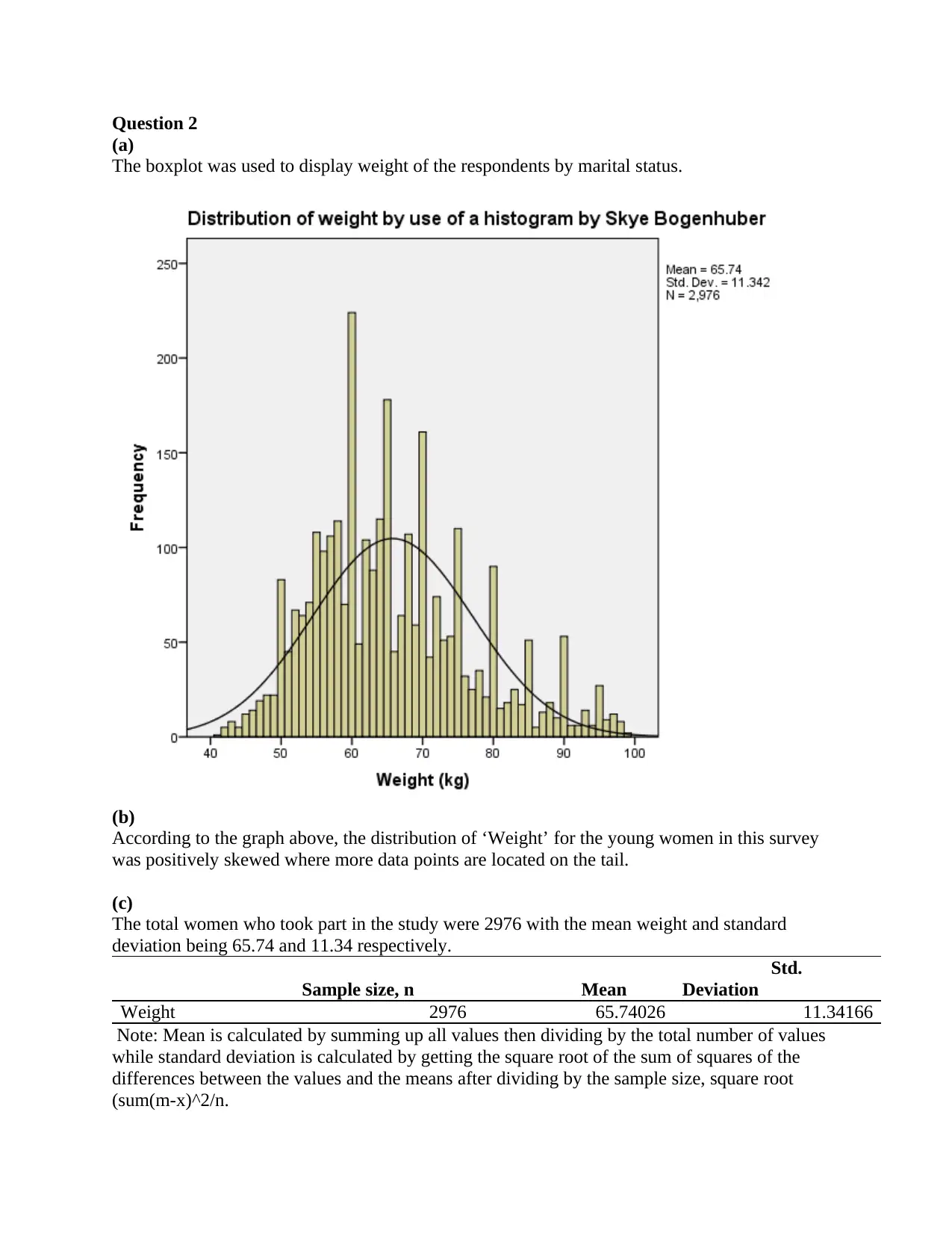
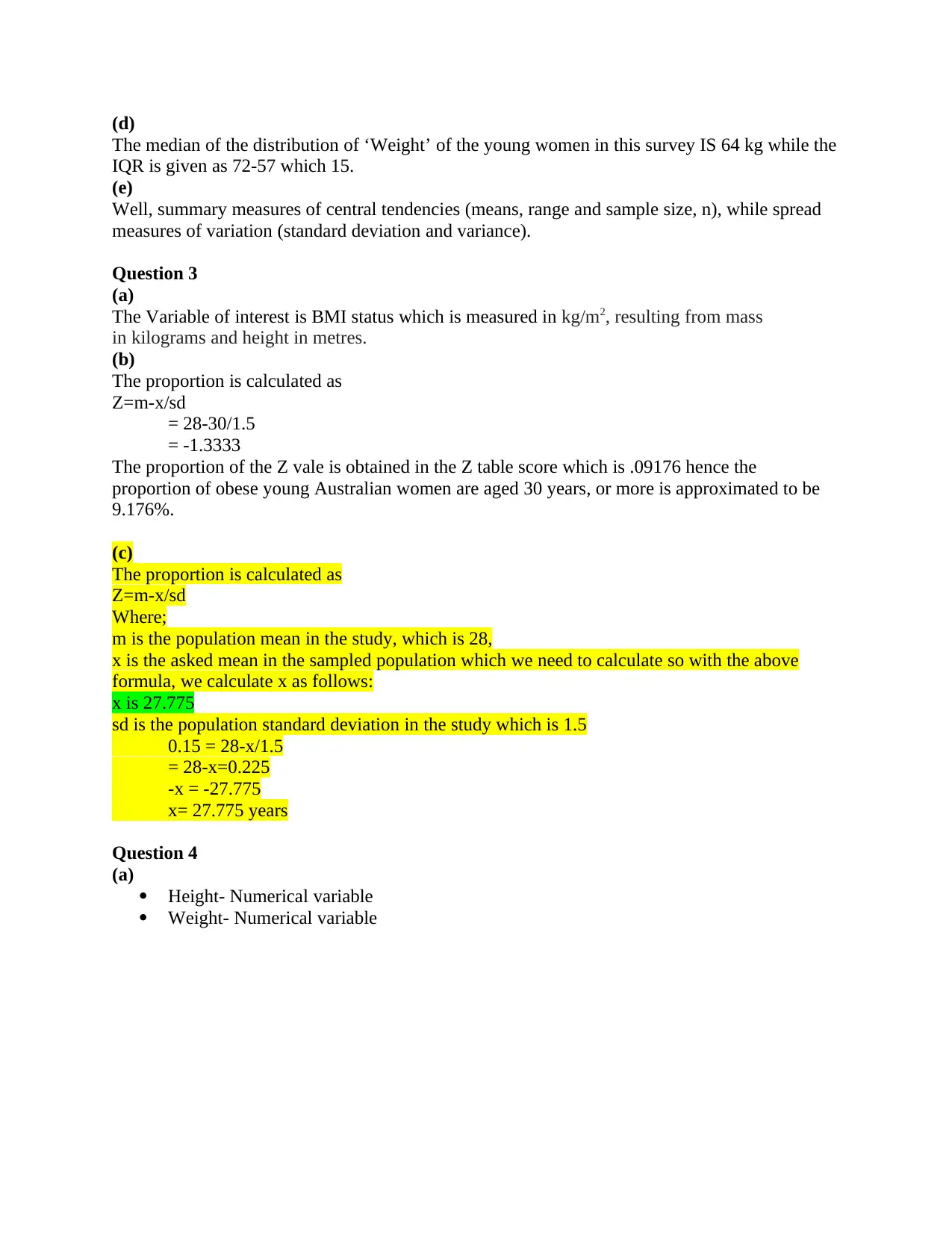
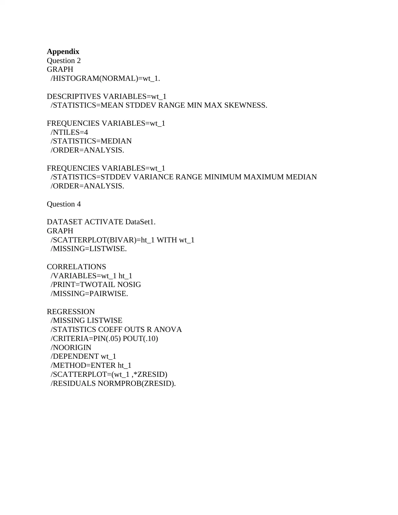
This document presents the solutions to STA2300 Data Analysis Assignment 1, covering various statistical concepts and methods. The assignment analyzes data using boxplots, correlation, regression analysis, and binomial distribution, and includes the interpretation of SPSS output. The solution addresses questions related to the distribution of weight, calculation of proportions, correlation between height and weight, regression equation, model parameters, and experimental study design. It also addresses potential confounders and the interpretation of study findings. The solutions provide detailed explanations and calculations, demonstrating a comprehensive understanding of the statistical concepts and their practical application.

Question 2
(a)
The boxplot was used to display weight of the respondents by marital status.
(b)
According to the graph above, the distribution of ‘Weight’ for the young women in this survey
was positively skewed where more data points are located on the tail.
(c)
The total women who took part in the study were 2976 with the mean weight and standard
deviation being 65.74 and 11.34 respectively.
Sample size, n Mean
Std.
Deviation
Weight 2976 65.74026 11.34166
Note: Mean is calculated by summing up all values then dividing by the total number of values
while standard deviation is calculated by getting the square root of the sum of squares of the
differences between the values and the means after dividing by the sample size, square root
(sum(m-x)^2/n.

(d)
The median of the distribution of ‘Weight’ of the young women in this survey IS 64 kg while the
IQR is given as 72-57 which 15.
(e)
Well, summary measures of central tendencies (means, range and sample size, n), while spread
measures of variation (standard deviation and variance).
Question 3
(a)
The Variable of interest is BMI status which is measured in kg/m2, resulting from mass
in kilograms and height in metres.
(b)
The proportion is calculated as
Z=m-x/sd
= 28-30/1.5
= -1.3333
The proportion of the Z vale is obtained in the Z table score which is .09176 hence the
proportion of obese young Australian women are aged 30 years, or more is approximated to be
9.176%.
(c)
The proportion is calculated as
Z=m-x/sd
Where;
m is the population mean in the study, which is 28,
x is the asked mean in the sampled population which we need to calculate so with the above
formula, we calculate x as follows:
x is 27.775
sd is the population standard deviation in the study which is 1.5
0.15 = 28-x/1.5
= 28-x=0.225
-x = -27.775
x= 27.775 years
Question 4
(a)
 Height- Numerical variable
 Weight- Numerical variable

(b)
For to note, r is the square root of the R square which automatically come with the recession line
graph. So, r= sqrt (0.098) which is 0.314.
(c)
By visualizing the above scatterplot, there is a weak positive relationship between height and
weight of the women as indicated by the r=0.314 which is the square root of R SQUARE
ABOVE; 0.098. However, the direction is that as height increases, the weight also increases.
Looking at the graph, there seems to be no noticeable existence of outliers.
(d)
The Pearson correlation, r=0.314, p-value=0.0005<0.05 indicate the existence of a weak positive
association between height and weight of the women.
Correlations
Weight Height
wt_1
Pearson Correlation 1 .314**
Sig. (2-tailed) .000
N 2976 2976
ht_1
Pearson Correlation .314** 1
Sig. (2-tailed) .000
N 2976 2976
**. Correlation is significant at the 0.01 level (2-tailed).
(e)
𝑦 ̂ = 𝑏0 + 𝑏1𝑥 (1)
From the above equation, the regress and (y) is the weight and the regressor x is the height. On
the other hand, 𝑦 ̂ is the predicted weight. To note, weight is chosen to be the regress mainly
because it is the variable to be predicted in the research question. The height, in this case, is the
regressor because it is the variable that will be used to predict the regress. The equation 8.5714 *
x + 65.7143 is also automatically generated in SPSS output and come with the regression line
and it represents the weight of all the 2976 sample size.
X is the provided height to be predicted which in this case is 165cm so it is 8.5714 multiply by
165 plus 65.7143

(f)
Predicted weight is 8.5714 * 165 + 65.7143 which is 1480kg. this is not accurate prediction since
the prediction model accuracy value is low just only 9% as indicated by the R squared value in
the graph.
(g)
Proportion of the variability in weight for young women can be explained by the model is 0.098
which is 9.8% as shown by the value of R square in the chart.
Question 5
(a)
Model Parameter Value
Bar chart Number of bars (n) 70
Men Age Weight
0
20
40
60
80
100
120
140
160
180
BarChart

(b)
Age, gender, and weight can fit in the model given that the number values can easily be
displayed in the chart.
(c)
* refers to multiplication sign, the numbers were obtained from the question itself
Proportion is 70% which is equivalent to 70/100=0.7
Mean is proportion multiply by age which is given as below
mean= 0.7*18
mean = 5.6
s.d= value of the proportion which is 1.32 and this was extracted from the analysis.
(d)
Probability= 15/20
=0.75
(e)
Pr= 75/100
=0.75
The assumption is that there is a binominal distribution. A Binomial Distribution shows either
(S)uccess or (F)ailure. x = total number of “successes” (pass or fail, heads or tails etc.)
Question 6
(a)
This was an experimental study because there was introduction of a treatment where the
researchers after recruiting 33 overweight and obese adults, aged between 23 and 59, they
randomly assigned them to receive supplements of L-glutamine or L-alanine for two weeks.
(b)
 Intervention group which is either receiving supplements of L-glutamine or L-alanine
 Weight
 Duration which is two weeks
(c)
Basically, a confounder is a variable with ability to influence the outcome, more so the
dependent and independent variables, which may cause a false association, (Wang, et, al, 2017).
One plausible confounding variable in this study was the age range of the volunteers which was
large (23-59 years) and aging may influence intestinal microbiota. To over come this, the age
group should be among the young populations like 25-35 years.
(d)
No, these findings suggest that oral supplementation of L-glutamine have similar effects on gut
microbiota as weight loss,” said the researchers and that the results obtained in this study were
statistically significant”. This was not reflected in the title of the article “L-Glutamine changes
gut bacteria leading to weight loss.”

References
Wang, J., Zhao, Q., Hastie, T., & Owen, A. B. (2017). Confounder adjustment in multiple
hypothesis testing. Annals of statistics, 45(5), 1863.

Appendix
Question 2
GRAPH
/HISTOGRAM(NORMAL)=wt_1.
DESCRIPTIVES VARIABLES=wt_1
/STATISTICS=MEAN STDDEV RANGE MIN MAX SKEWNESS.
FREQUENCIES VARIABLES=wt_1
/NTILES=4
/STATISTICS=MEDIAN
/ORDER=ANALYSIS.
FREQUENCIES VARIABLES=wt_1
/STATISTICS=STDDEV VARIANCE RANGE MINIMUM MAXIMUM MEDIAN
/ORDER=ANALYSIS.
Question 4
DATASET ACTIVATE DataSet1.
GRAPH
/SCATTERPLOT(BIVAR)=ht_1 WITH wt_1
/MISSING=LISTWISE.
CORRELATIONS
/VARIABLES=wt_1 ht_1
/PRINT=TWOTAIL NOSIG
/MISSING=PAIRWISE.
REGRESSION
/MISSING LISTWISE
/STATISTICS COEFF OUTS R ANOVA
/CRITERIA=PIN(.05) POUT(.10)
/NOORIGIN
/DEPENDENT wt_1
/METHOD=ENTER ht_1
/SCATTERPLOT=(wt_1 ,*ZRESID)
/RESIDUALS NORMPROB(ZRESID).