STA2300 Data Analysis Assignment S3 2019: Statistical Analysis Report

This document presents a comprehensive solution to the STA2300 Data Analysis assignment, focusing on various statistical concepts and their applications. The assignment explores an experimental study on the effect of caffeine on anxiety, identifying response and explanatory variables, and implementing experimental design principles. It then delves into the analysis of hypertension prevalence using a binomial distribution model, calculating probabilities and assessing assumptions. Furthermore, the solution analyzes hospital staff data using SPSS, including contingency tables, proportions, and associations. It also addresses the normal distribution, calculating proportions for kindergarten children's heights. Finally, the assignment concludes with regression analysis to predict total staff cost based on total nurse cost, utilizing SPSS to generate and interpret the results.

Surname 1
Student’s Name
Instructor’s Name
Course
Date
STA2300 Data Analysis S3, 2019
Question 1 (16 marks)
A professor conducted a study on the effect of the amount of caffeine on anxiety. Of the 60
subjects available for the study, 20 were randomly assigned to Group 1 (giving 2 cups of
decaffeinated coffee with 0mg caffeine), another 20 were randomly assigned to Group 2 (giving
2 cups of coffee with 2mg caffeine), and the remaining 20 were assigned to Group 3 (giving 2
cups of coffee with 6mg caffeine).
After 30 minutes of consumption of the three types of coffee mixtures by the three different
groups each of the subjects were given a test that measures their level of perceived anxiety.
For the above study, answer the following questions.
(a) (2 marks) Is the above study observational or experimental? In less than 50 words clearly
explain your choice based on the extract given above.
This is an experimental research study-This involves collection of data and developing findings
to support or reject the null hypothesis. This is shown since the study seeks to establish effect of
caffeine on anxiety. Different measures of caffeine are given to subjects who were randomly
selected.
(b) (2 marks) Identify and write down the name of the response variable(s) and explanatory
variable(s) of interest.
Response variable/dependent variable-level of anxiety.
Explanatory variable/independent variable-caffeine amounts.
(c) (3 marks).How many levels of the explanatory variable are in the study? Clearly describe all
the levels.
The explanatory variable (caffeine amounts) is divided into 3 levels;
Level 1-decaffeinated coffee with 0mg caffeine
Level 2- 2 cups of coffee with 2mg caffeine

Surname 2
Level 3- 2 cups of coffee with 6mg caffeine
(d) (2 marks) Explain why, or why not, Group 1 can be treated as a ‘placebo’ group in the
context of the study.
Group 1 is treated as the placebo or control since the subjects are not given any caffeine
treatment. The decaffeinated coffee have no amounts of caffeine hence is the control group.
(e) (4 marks) Explain which principles of experimental design were implemented, and how, in
the study?
Probability sampling was implemented. Subjects were randomly assigned to either of the
three groups. All data in an experimental research must be quantified, or measured. Caffeine
levels are measured and assigned as 0mg, 2mg and 6mg.In addition, a placebo/control group is
an important principle in experimental design since it shows if the treatment had significant
influence on the response variable.
(f) (3 marks) Explain what is meant by an experimental unit. Identify the experimental units in
the context of the study. How many experimental units are used in the study?
An experimental unit is the physical entity which can be assigned a treatment randomly.
In this experiment, each individual among the sample size of 60 is an experimental unit. A total
of 60 experimental units are used in the study.
Question 2 (18 marks)
Hypertension (high blood pressure) is a common health problem amongst the Australian
population. It is the greatest contributor to the burden of cardiovascular disease (CVD).
According to Australian Heart Foundation data, 25% Australians of aged between 45-54 years
suffer from hypertension. To investigate how Australians are affected by the incidence of
hypertension, a researcher selected a random sample of 12 Australians of the above age group.
Use this information to answer the following questions:
(a) (2 marks).Suggest an appropriate model to estimate the probabilities of the number of
Australians of the above age group (45-54 years) who have a hypertension. What are the
parameters of this model?
The binomial distribution model can be used to estimate the probabilities of the number of
Australians of the above age group (45-54 years) who have a hypertension
(b) (4 marks).Explain why this model is appropriate by discussing the important distinguishing
features of the model, focusing on the underlying conditions for the validity of the model.
The distribution can be thought of as simply the probability of a having a success or failure of the
outcome of an event. In this case, suffering hypertension could be thought has a probability of
success.

Surname 3
(c) (2 marks) Using the model from part (a), estimate the probability that, in the randomly
selected sample of 12 Australians of the above age group, at most 3 will have hypertension.
P=0.25 and q=1-0.25=0.75
In this case x=3 and n=12
This is a binomial distribution with formula p(x) = C(n,x) * p^x * q^(n-x)
P(X=<3)=P(X=0)+ P(X=1)+ P(X=2)+ P(X=3)
=0.03168+0.12671+0.23229+0.2581= 0.64878
(d) (4 marks) A random sample of 120 Australians of the above age group have been selected to
have their hypertension checked. For this sample of 120, estimate the mean and standard
deviation of the number of Australians with hypertension.
Mean=E(X)=np=120*.25=30
Standard deviation =npq=120*.25*(1-.25)=22.5
(e) (4 marks) Determine the probability that, in the random sample of 120 Australians of the age
group (selected in part (c)), 20 or more will have hypertension.
P=0.25 and q=1-0.25=0.75
In this case x=20 and n=120
This is a binomial distribution with formula p(x) = C(n,x) * p^x * q^(n-x)
P(X>=20)= 0.98925
(f) (2 marks) State and check any assumptions, conditions or rules of thumb that should be
considered for the validity of the result obtain in part (e).
The underlying assumptions of the binomial distribution are;
 There exists only one outcome for each trial
 Each of the each trial has the same probability of success
 Each trial is independent of each other.
Question 3 (14 marks)
This question uses information from the data file HospitalStaff.sav found under the Assignments
and Datasets link on the StudyDesk (also see HospitalStaff.txt for more details about the health

Surname 4
study and the variables measured). Make sure the variable view in SPSS is setup correctly with
all ‘labels’ correctly defined (with units), all ‘values’ assigned correctly for categorical variables
and the correct ‘measure’ selected for all variables.
As a researcher you are seeking to gain insights into the variables measured in this study. You
are interested in ascertaining if there is any relationship between Region of hospital location and
presence of Obstetrics wards.
(a) (4 marks) Using SPSS, produce a contingency table to display the relationship between
HospRegion (region of hospital) and the presence of an Obstetrics wards in this study. The title
for this table should reflect the table contents and also include your name. (Note that a table title
should appear above the table). You can copy and paste this table straight into your assignment;
just ensure you have a meaningful title.
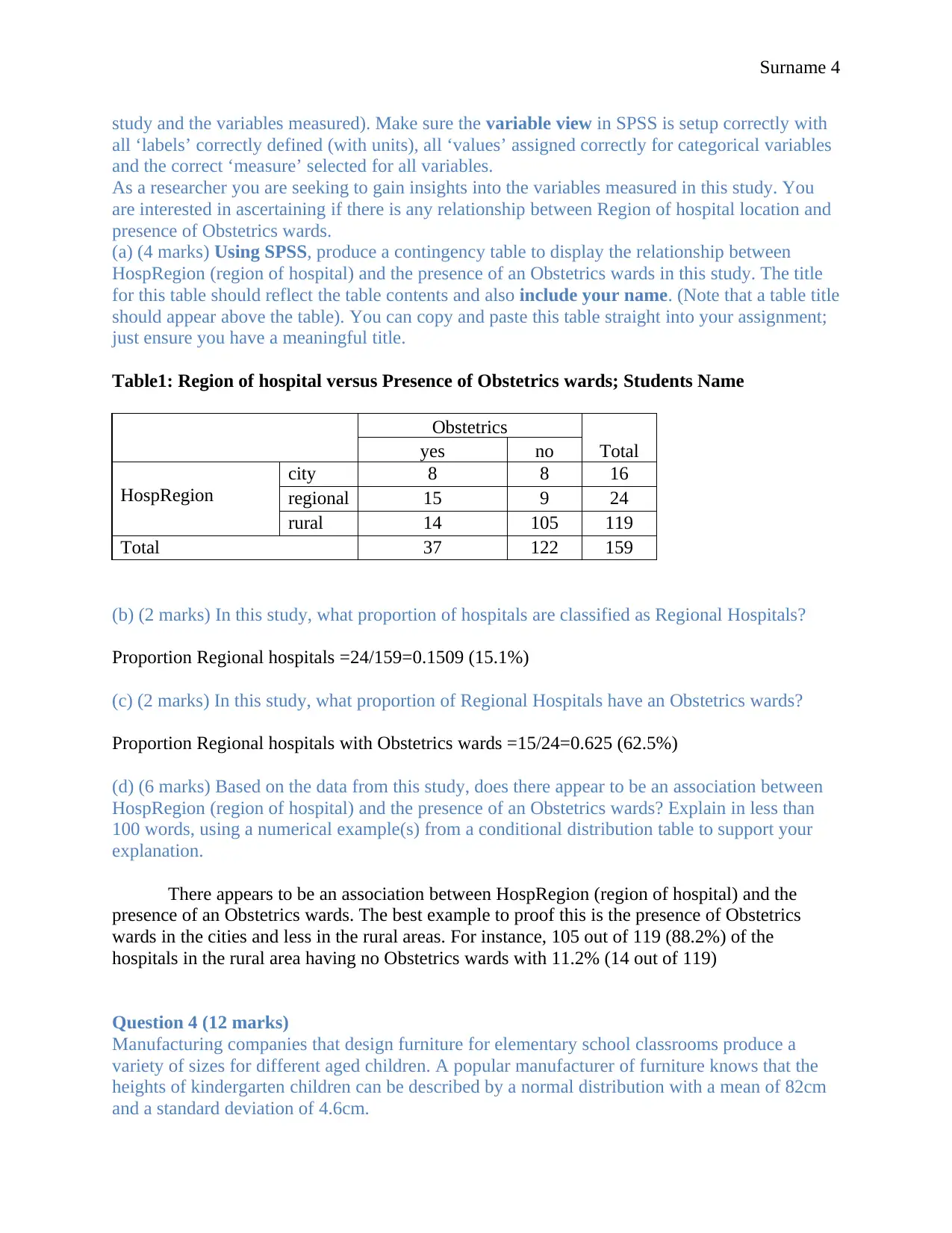
Table1: Region of hospital versus Presence of Obstetrics wards; Students Name
Obstetrics
Totalyes no
HospRegion
city 8 8 16
regional 15 9 24
rural 14 105 119
Total 37 122 159
(b) (2 marks) In this study, what proportion of hospitals are classified as Regional Hospitals?
Proportion Regional hospitals =24/159=0.1509 (15.1%)
(c) (2 marks) In this study, what proportion of Regional Hospitals have an Obstetrics wards?
Proportion Regional hospitals with Obstetrics wards =15/24=0.625 (62.5%)
(d) (6 marks) Based on the data from this study, does there appear to be an association between
HospRegion (region of hospital) and the presence of an Obstetrics wards? Explain in less than
100 words, using a numerical example(s) from a conditional distribution table to support your
explanation.
There appears to be an association between HospRegion (region of hospital) and the
presence of an Obstetrics wards. The best example to proof this is the presence of Obstetrics
wards in the cities and less in the rural areas. For instance, 105 out of 119 (88.2%) of the
hospitals in the rural area having no Obstetrics wards with 11.2% (14 out of 119)
Question 4 (12 marks)
Manufacturing companies that design furniture for elementary school classrooms produce a
variety of sizes for different aged children. A popular manufacturer of furniture knows that the
heights of kindergarten children can be described by a normal distribution with a mean of 82cm
and a standard deviation of 4.6cm.

Surname 5
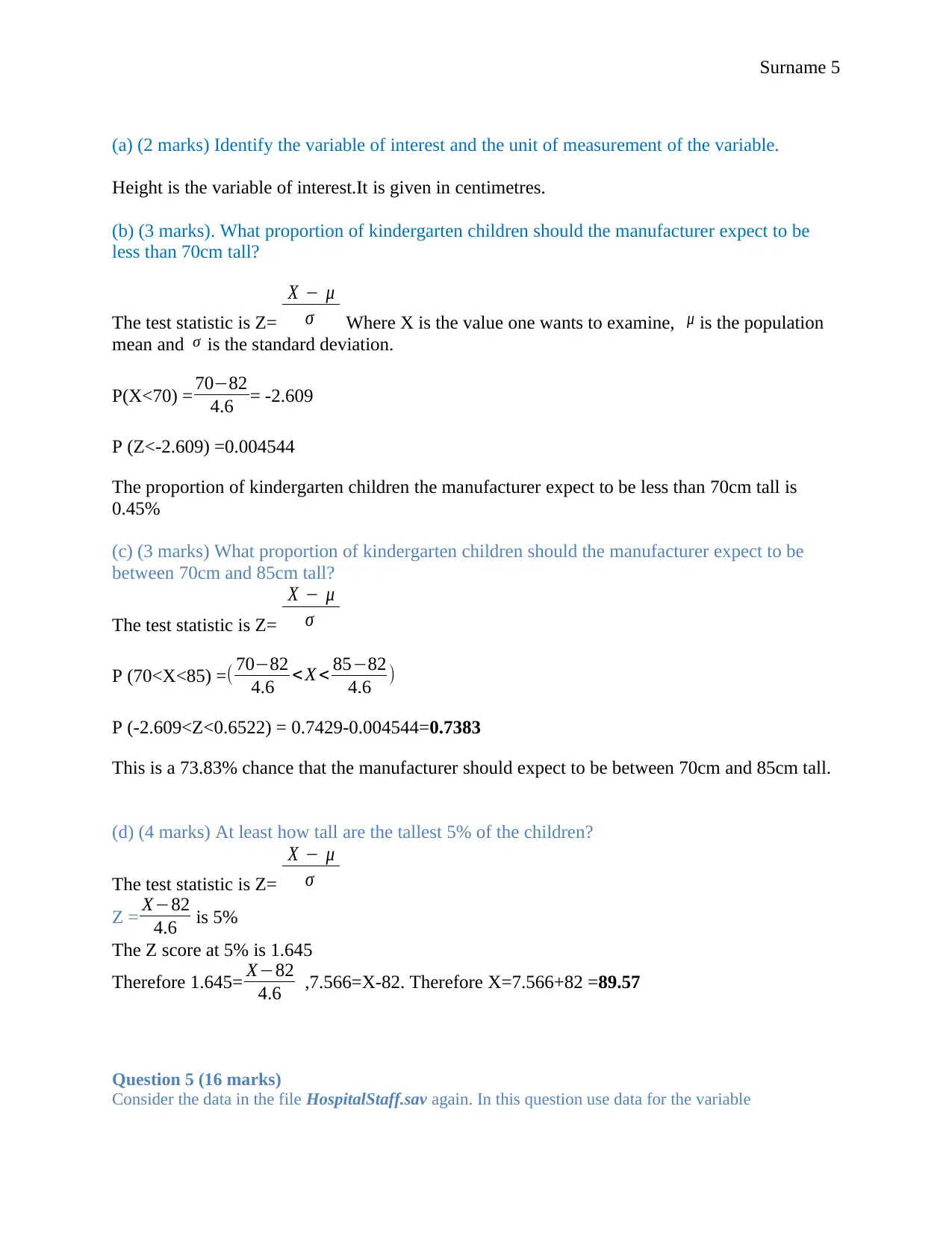
(a) (2 marks) Identify the variable of interest and the unit of measurement of the variable.
Height is the variable of interest.It is given in centimetres.
(b) (3 marks). What proportion of kindergarten children should the manufacturer expect to be
less than 70cm tall?
The test statistic is Z=
X − μ
σ Where X is the value one wants to examine, μ is the population
mean and σ is the standard deviation.
P(X<70) = 70−82
4.6 = -2.609
P (Z<-2.609) =0.004544
The proportion of kindergarten children the manufacturer expect to be less than 70cm tall is
0.45%
(c) (3 marks) What proportion of kindergarten children should the manufacturer expect to be
between 70cm and 85cm tall?
The test statistic is Z=
X − μ
σ
P (70<X<85) =( 70−82
4.6 < X < 85−82
4.6 )
P (-2.609<Z<0.6522) = 0.7429-0.004544=0.7383
This is a 73.83% chance that the manufacturer should expect to be between 70cm and 85cm tall.
(d) (4 marks) At least how tall are the tallest 5% of the children?
The test statistic is Z=
X − μ
σ
Z = X−82
4.6 is 5%
The Z score at 5% is 1.645
Therefore 1.645= X−82
4.6 ,7.566=X-82. Therefore X=7.566+82 =89.57
Question 5 (16 marks)
Consider the data in the file HospitalStaff.sav again. In this question use data for the variable

Surname 6
Enrolnurses2012 (2012 Paid full time equivalent enrolled nurses).
Use SPSS to find the answers to the following questions, but do not copy and paste SPSS output into your
answer for parts (c) and (d) (make sure you always include units where appropriate).
(a) (5 marks) Display the distribution of Enrolnurses2012 in this study, using an appropriate graph. Label
the axes correctly, include units of measure and provide an appropriate title. Include your name in the
title of your graph.
(b) (4 marks) Using the graph in (a) only (don’t refer to SPSS summary statistics), describe in no more
than 60 words, the distribution of Enrolnurses2012. Include comments on shape, centre and spread of the
distribution and the existence of outliers, if any. Do not include information from any calculations, use the
graph only.
The histogram above shows that the data is not normally distributed but positively skewed. This is where
a longer tail is observed on the right hand side compared to the left. In the case above the median value is
certainly smaller than the mean value. No outlier were realized. Few nurses were paid full time.
(c) (3 marks) What is the sample size, mean and standard deviation of the distribution of
Enrolnurses2012 in the study? (Use SPSS, but do not just copy/paste SPSS output).

Surname 7
According to the results generated, a sample of 159 individual were involved in the study. The
mean and standard deviation of the distribution of Enrolnurses2012 was 16.81 and 32.698 respectively.
(d) (2 marks) Using SPSS find the median and inter quartile range (IQR) of the distribution of
Enrolnurses2012 in the study? (Do not copy/paste SPSS output).
The median of the distribution of Enrolnurses2012 was 5.40 units. The first and third quartile value were
0.85 and 12.19 respectively.
Therefore IQR=Q3-Q1=12.19-0.85=11.34
(e) (2 marks) For the distribution of Enrolnurses2012 in part (a), which statistics are appropriate to
measure its centre and spread? Give a reasonable explanation for your choice.
The mode and standard deviation are best measures for central tendency and spread respectively.
Mode will be best measure since these are observations. The standard deviation will also reveal
the spread of the data
Question 6 (24 marks)
Consider the data in the file HospitalStaff.sav again. As a researcher you are interested in seeing
if TotalNurseCost can be used effectively to predict TotalStaffCost, for the hospitals included in
the study. Note that the variables TotalNurseCost and TotalStaffCost are expressed in million
Australian dollars (from the TotalNurseCost2012 and TotalStaffCost2012 respectively).
(a) (3 marks) What are the two variables you will need to include in your analysis? What type of
variables are they? What are the units of measurement of these variables?
Independent variable: TotalNurseCost
Dependent variable: TotalStaffCost
They are expressed in million Australian dollars
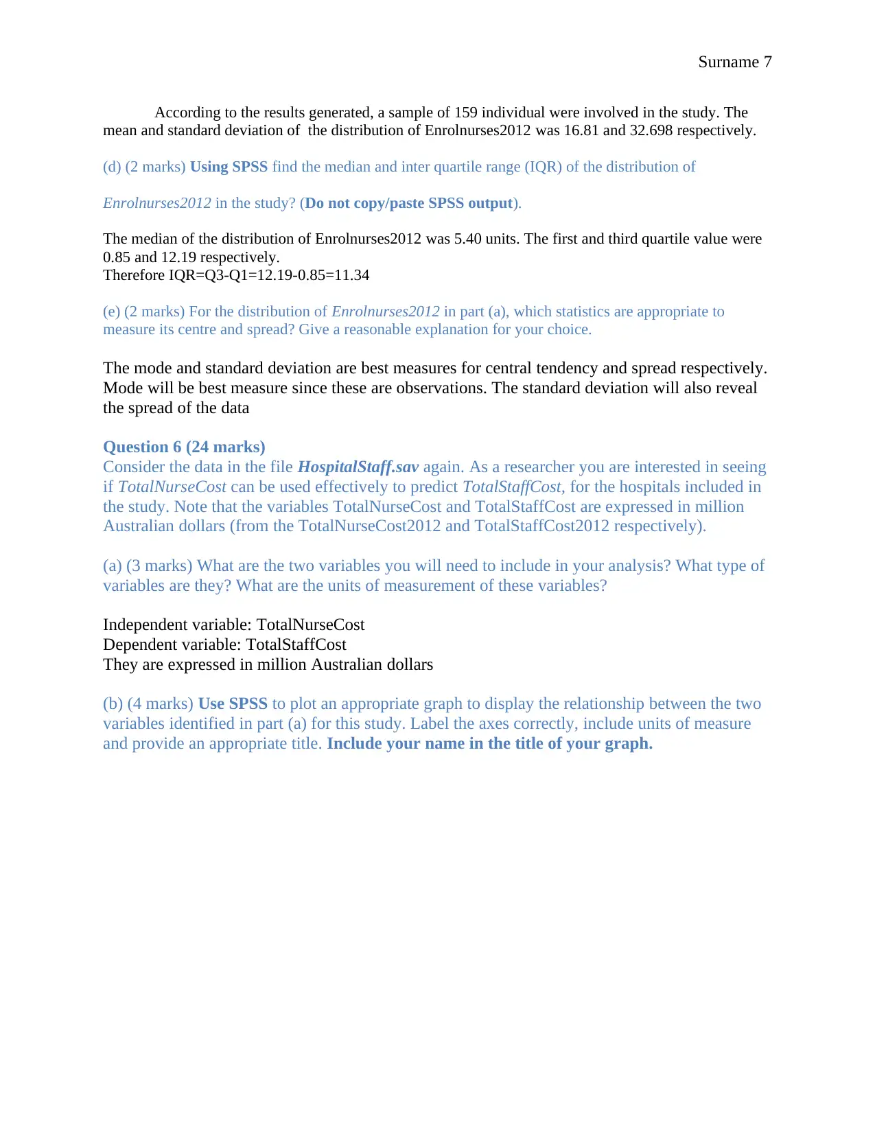
(b) (4 marks) Use SPSS to plot an appropriate graph to display the relationship between the two
variables identified in part (a) for this study. Label the axes correctly, include units of measure
and provide an appropriate title. Include your name in the title of your graph.

Surname 8
(c) (4 marks) From the graph in part (b), describe (in no more than 30 words) the form, direction
and scatter of this relationship, and identify any outliers.
There exist a strong positive relationship between total nurse cost and the total staff cost. This is
because as nurse cost increase, the staff cost increase and vice versa.
(d) (3 marks) Calculate an appropriate statistic to measure the strength and direction of the
relationship between the two variables for the study. Justify your choice of this statistic and
interpret what it tells about the relationship.
The Pearson Correlation coefficient is an appropriate statistic to measure the strength and
direction of the two variables. It ranges between -1 to +1,where negative value show a negative
relationship while the positive values show a positive relationship (Sullivan,20-98). Values near
+1 and -1 (>.5) show strong relationship while value between 0.3 to 0.4 show moderate strong
relationship. Value near 0 show weak relationship with a value of 0 showing no relationship. The
two values are continuous hence Pearson is the best measure

Surname 9
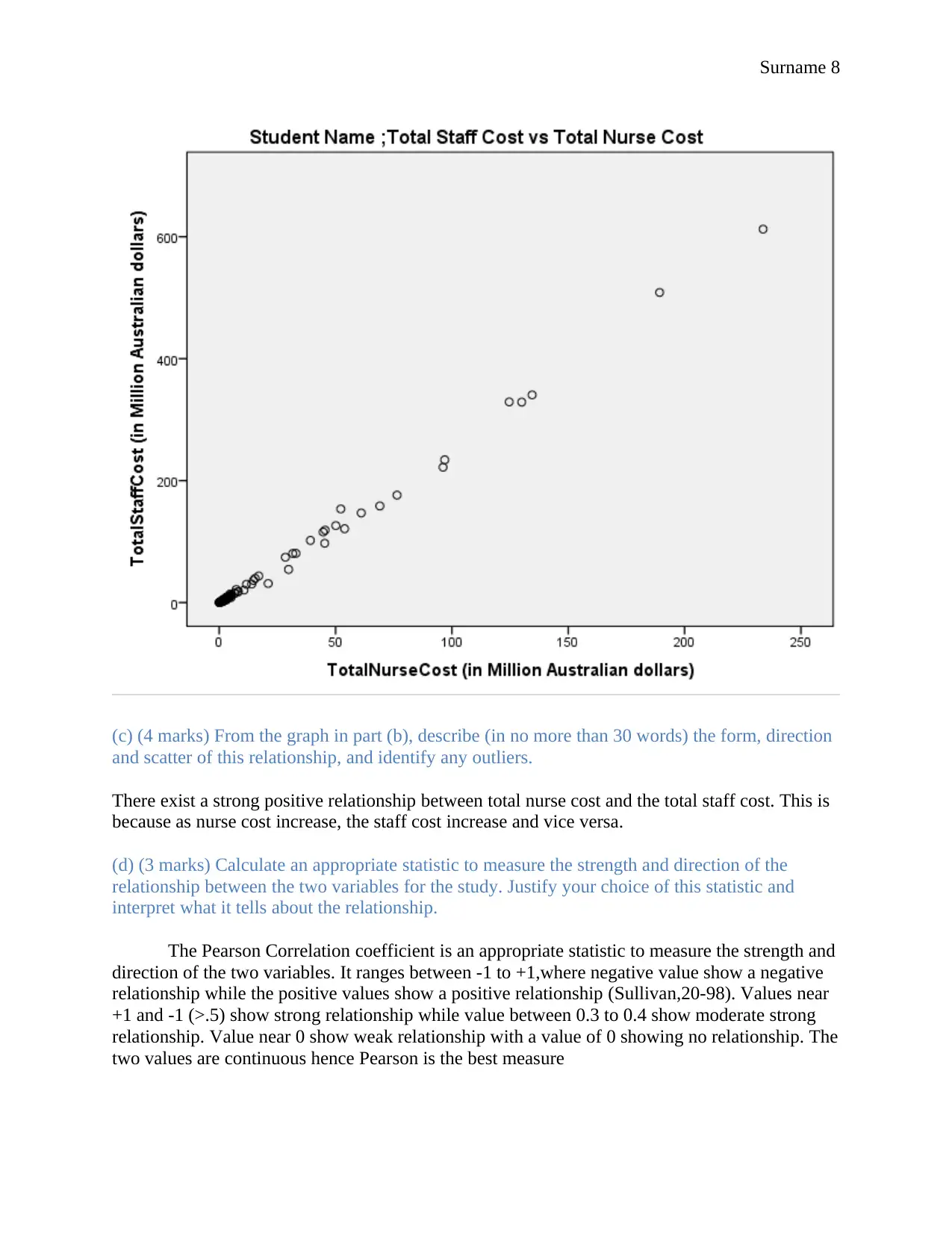
(e) (4 marks) Use SPSS to find the equation of the regression line which could be used to predict
the TotalStaffCost of a hospital for a given value of the TotalNurseCost of the same hospital.
State the equation of the linear regression line stating any symbols used.
The regression equation is expressed by y=β0+ β1 x + ε ; where ε is the error term
The regression model is y=-1.516+2.570x+e
The regression model is Total Staff Cost =-1.516+2.570(Total nurse cost)+e
The r=0.998 which show a strong positive relationship
The R-squared value is 0.996 implying that 99.6% of the variation in the model is
explained by the independent variable
(f) (2 marks) Plot the best fitted linear regression line on the graph in part (b).
(g) (2 marks) Interpret the value of the intercept and slope of the linear regression line in the
context of the question.

Surname 10
The y –intercept value is -1.516.This is where the line of best fir cuts the y-axis when the total
nurse cost is 0.The slope is 2.570.It is positive hence showing a positive relationship
(Holcomb,45). A unit increase in total nurse cost causes the staff cost to increase by 2.57 million
Australian dollars.
(h) (2 marks) Do you think this procedure is an appropriate method for predicting the
TotalStaffCost of a hospital when the value of TotalNurseCost of the same hospital is $300
million? Give two reasons to support your decision.
The regression model is Total Staff Cost =-1.516+2.570(Total nurse cost)
When the total nursing cost is $300,\
The regression equation become ;Total Staff Cost =-1.516+2.570(300)=$769.484
million
The procedure is appropriate since the R-squared value was 0.996 implying that 99.6%
of the variation in the model is explained by the total nursing cost. There is therefore little
contribution of other factors outside the model.

Surname 11
Work Cited
Holcomb, Zealure C. Fundamentals of descriptive statistics. Routledge, 2016.
Sullivan, Michael. Fundamentals of statistics. Vol. 200. Prentice Hall, 2011.