Statistics Assignment: Analysis of Startup Costs in Businesses

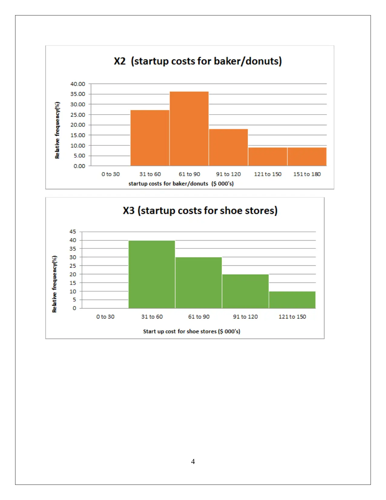
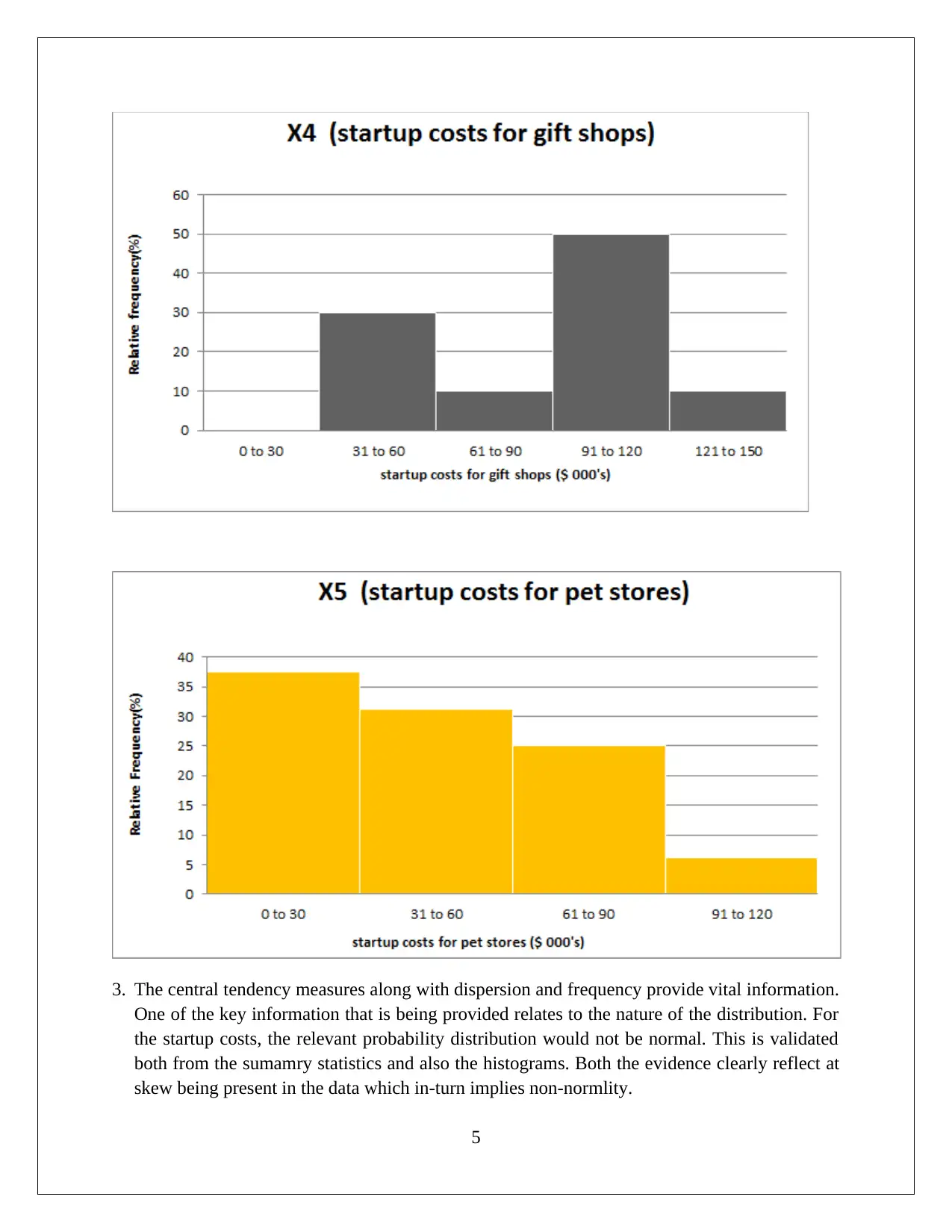
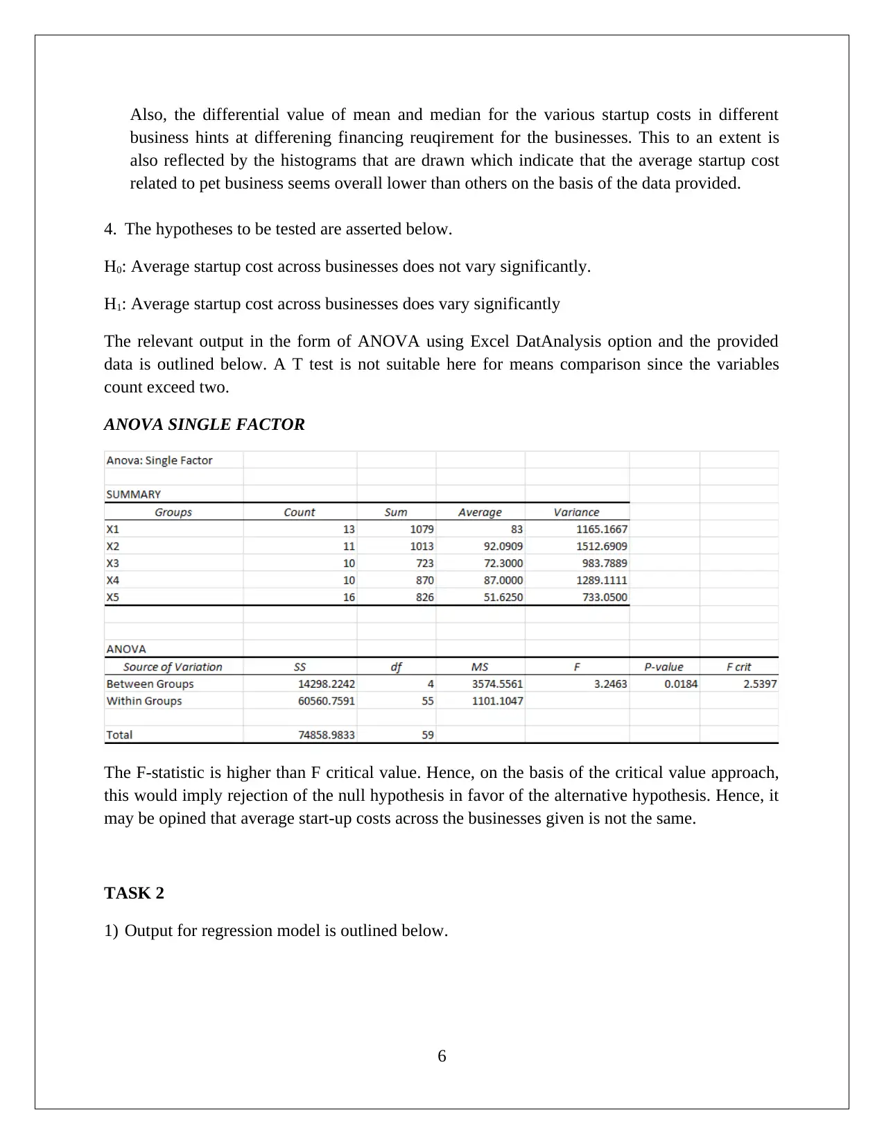
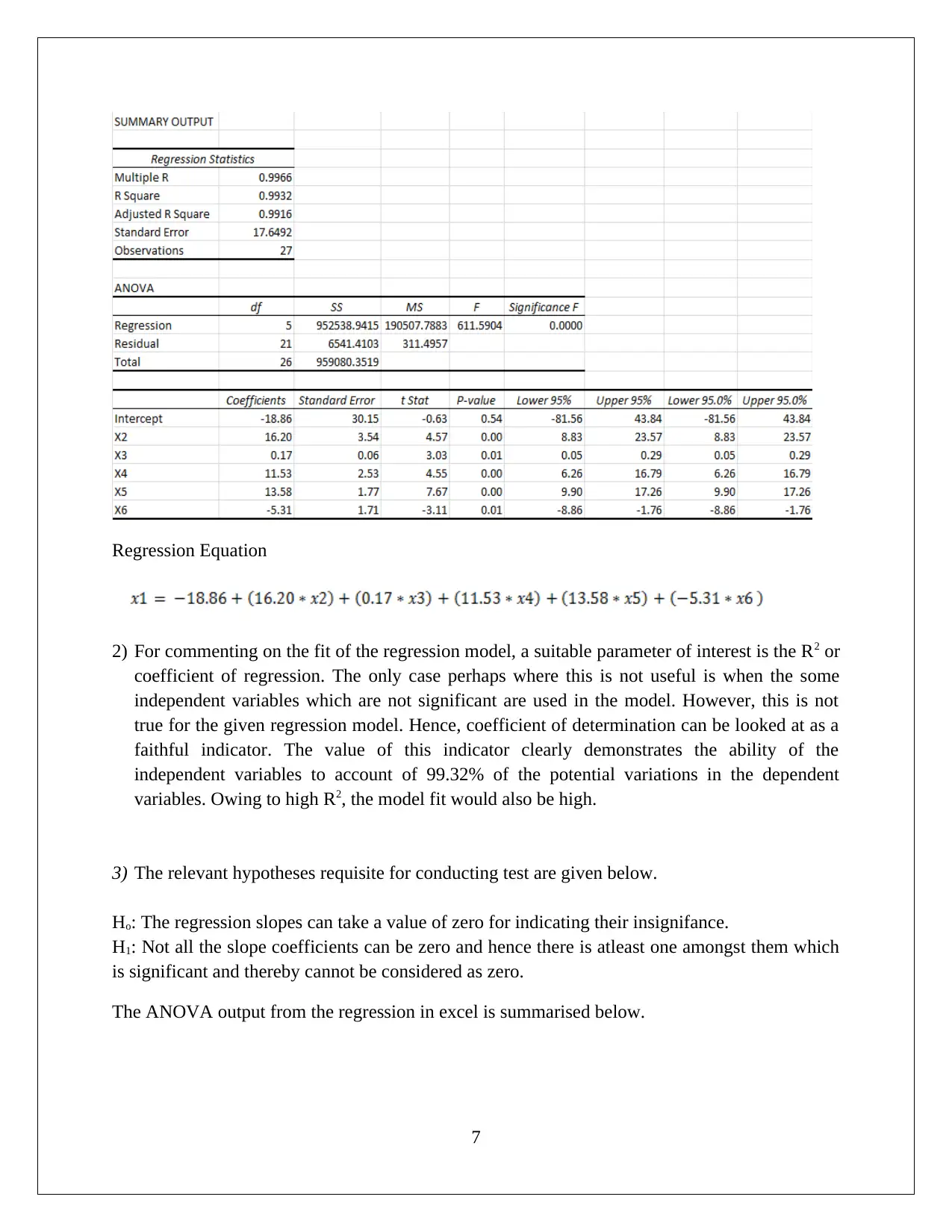
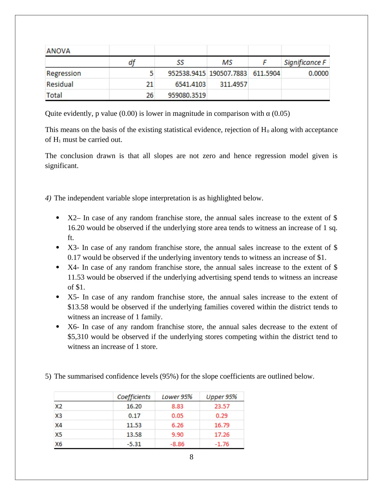
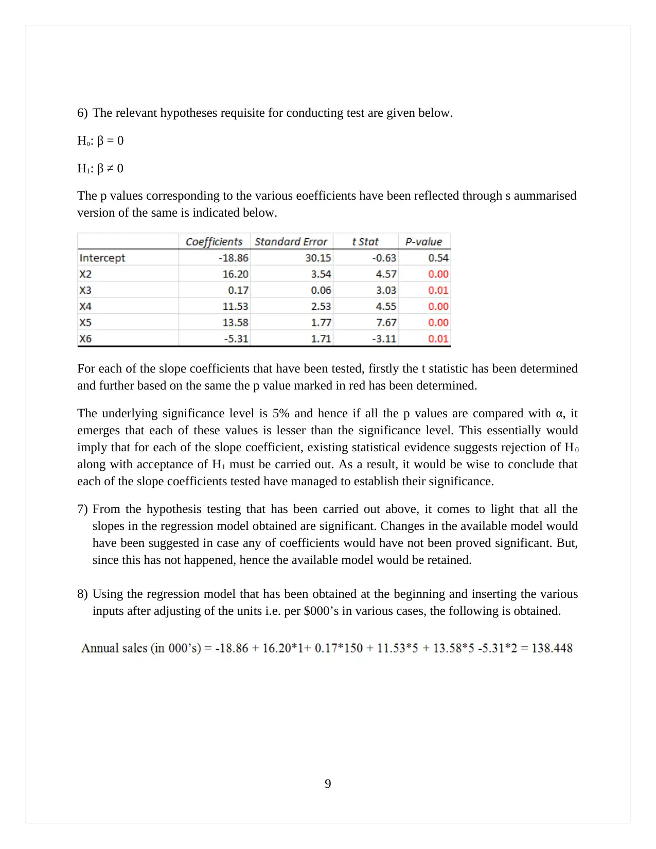
This statistics assignment analyzes startup costs across various businesses using frequency distribution tables and graphical representations to assess data normality and central tendency. The analysis includes hypothesis testing using ANOVA to compare average startup costs across different businesses, revealing significant variations. Additionally, a regression model is developed to explore the relationship between annual sales and various factors like store area, inventory, advertising spend, families covered, and competing stores. The regression model's high R-squared value indicates a strong fit, and hypothesis testing confirms the significance of all slope coefficients. The assignment provides detailed interpretations of the slope coefficients and confidence intervals, offering insights into how different variables impact sales. The student concludes that the model is significant and all slopes are significant.

STATISTICS
Student Id
[Pick the date]

Task 1
1. For the startup costs pertaining to different businesses, the specific indicators relating to the
central tendency along with the dispersion are summarised in the below outlined tables.
1

2. (a) The given data is presented in the form of frequency distribution tables.
2

(b) Taking the above frequency distribution tables into consideration, the following graphs
have been obtained.
3

4

3. The central tendency measures along with dispersion and frequency provide vital information.
One of the key information that is being provided relates to the nature of the distribution. For
the startup costs, the relevant probability distribution would not be normal. This is validated
both from the sumamry statistics and also the histograms. Both the evidence clearly reflect at
skew being present in the data which in-turn implies non-normlity.
5

Also, the differential value of mean and median for the various startup costs in different
business hints at differening financing reuqirement for the businesses. This to an extent is
also reflected by the histograms that are drawn which indicate that the average startup cost
related to pet business seems overall lower than others on the basis of the data provided.
4. The hypotheses to be tested are asserted below.
H0: Average startup cost across businesses does not vary significantly.
H1: Average startup cost across businesses does vary significantly
The relevant output in the form of ANOVA using Excel DatAnalysis option and the provided
data is outlined below. A T test is not suitable here for means comparison since the variables
count exceed two.
ANOVA SINGLE FACTOR
The F-statistic is higher than F critical value. Hence, on the basis of the critical value approach,
this would imply rejection of the null hypothesis in favor of the alternative hypothesis. Hence, it
may be opined that average start-up costs across the businesses given is not the same.
TASK 2
1) Output for regression model is outlined below.
6

Regression Equation
2) For commenting on the fit of the regression model, a suitable parameter of interest is the R2 or
coefficient of regression. The only case perhaps where this is not useful is when the some
independent variables which are not significant are used in the model. However, this is not
true for the given regression model. Hence, coefficient of determination can be looked at as a
faithful indicator. The value of this indicator clearly demonstrates the ability of the
independent variables to account of 99.32% of the potential variations in the dependent
variables. Owing to high R2, the model fit would also be high.
3) The relevant hypotheses requisite for conducting test are given below.
Ho: The regression slopes can take a value of zero for indicating their insignifance.
H1: Not all the slope coefficients can be zero and hence there is atleast one amongst them which
is significant and thereby cannot be considered as zero.
The ANOVA output from the regression in excel is summarised below.
7

Quite evidently, p value (0.00) is lower in magnitude in comparison with α (0.05)
This means on the basis of the existing statistical evidence, rejection of H0 along with acceptance
of H1 must be carried out.
The conclusion drawn is that all slopes are not zero and hence regression model given is
significant.
4) The independent variable slope interpretation is as highlighted below.
 X2– In case of any random franchise store, the annual sales increase to the extent of $
16.20 would be observed if the underlying store area tends to witness an increase of 1 sq.
ft.
 X3- In case of any random franchise store, the annual sales increase to the extent of $
0.17 would be observed if the underlying inventory tends to witness an increase of $1.
 X4- In case of any random franchise store, the annual sales increase to the extent of $
11.53 would be observed if the underlying advertising spend tends to witness an increase
of $1.
 X5- In case of any random franchise store, the annual sales increase to the extent of
$13.58 would be observed if the underlying families covered within the district tends to
witness an increase of 1 family.
 X6- In case of any random franchise store, the annual sales decrease to the extent of
$5,310 would be observed if the underlying stores competing within the district tend to
witness an increase of 1 store.
5) The summarised confidence levels (95%) for the slope coefficients are outlined below.
8

6) The relevant hypotheses requisite for conducting test are given below.
Ho: β = 0
H1: β ≠ 0
The p values corresponding to the various eoefficients have been reflected through s aummarised
version of the same is indicated below.
For each of the slope coefficients that have been tested, firstly the t statistic has been determined
and further based on the same the p value marked in red has been determined.
The underlying significance level is 5% and hence if all the p values are compared with α, it
emerges that each of these values is lesser than the significance level. This essentially would
imply that for each of the slope coefficient, existing statistical evidence suggests rejection of H0
along with acceptance of H1 must be carried out. As a result, it would be wise to conclude that
each of the slope coefficients tested have managed to establish their significance.
7) From the hypothesis testing that has been carried out above, it comes to light that all the
slopes in the regression model obtained are significant. Changes in the available model would
have been suggested in case any of coefficients would have not been proved significant. But,
since this has not happened, hence the available model would be retained.
8) Using the regression model that has been obtained at the beginning and inserting the various
inputs after adjusting of the units i.e. per $000’s in various cases, the following is obtained.
9