STAT100: Exploring Bike Sharing Trends Through Statistical Analysis

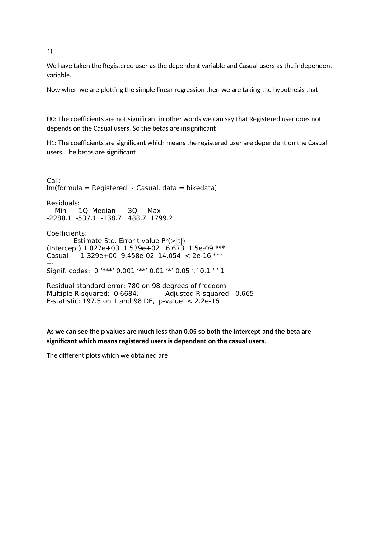
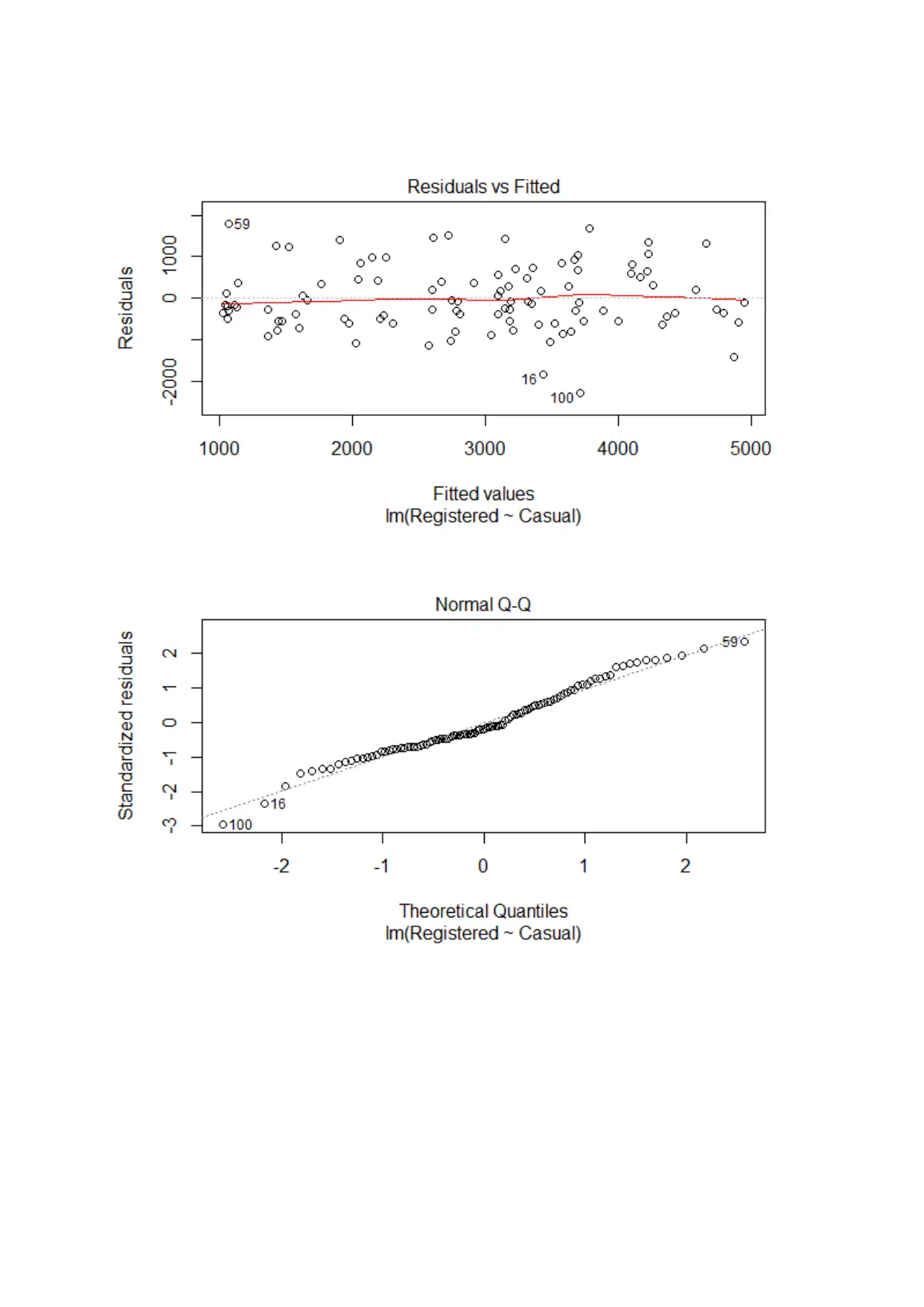
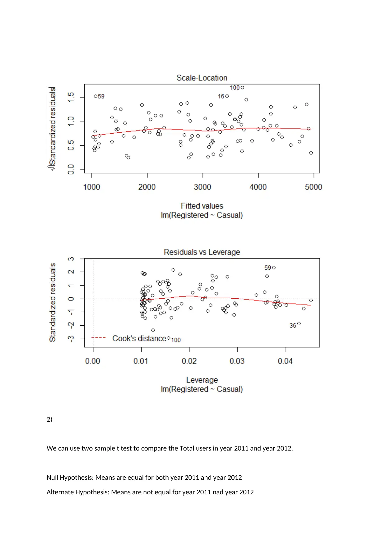
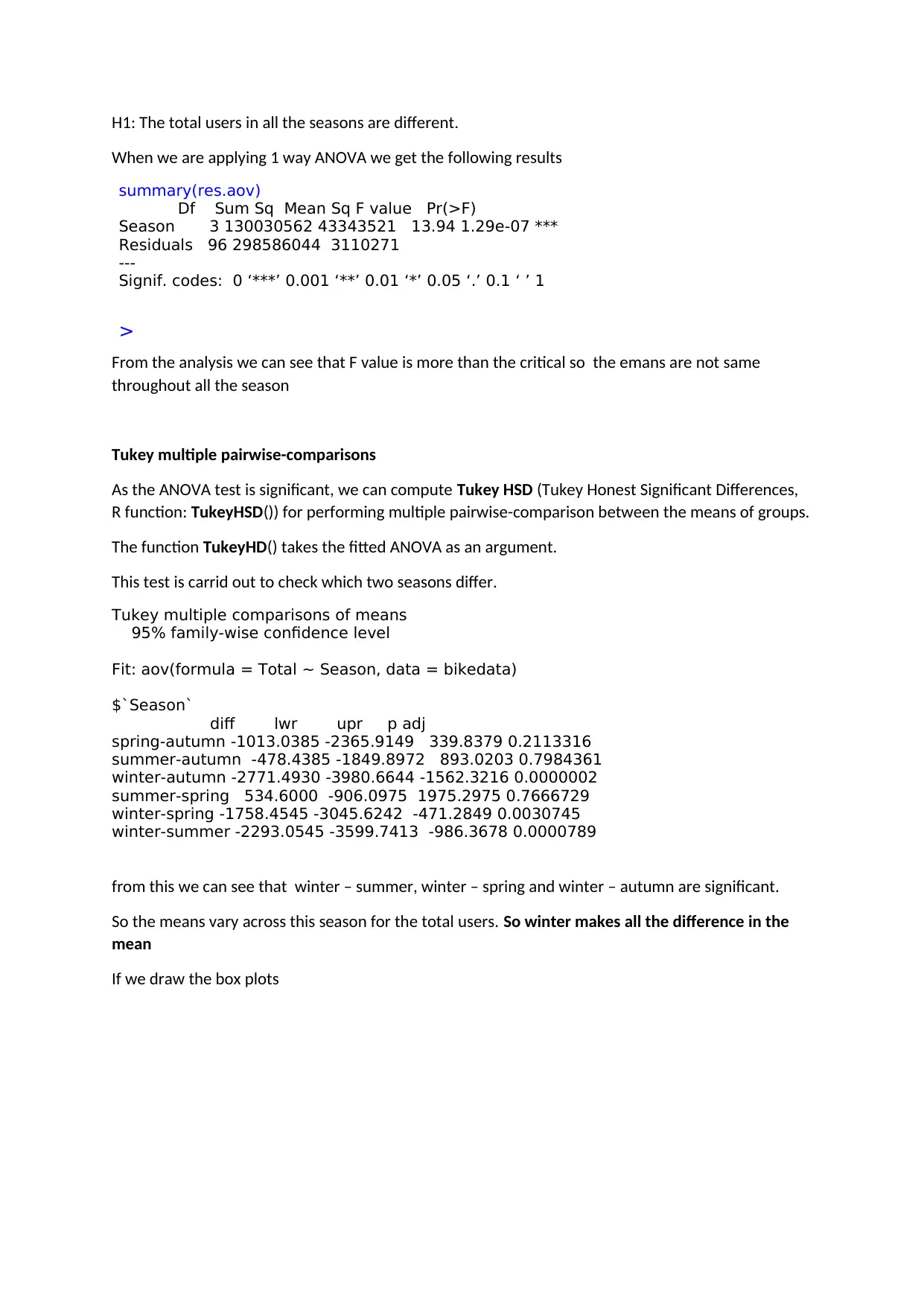
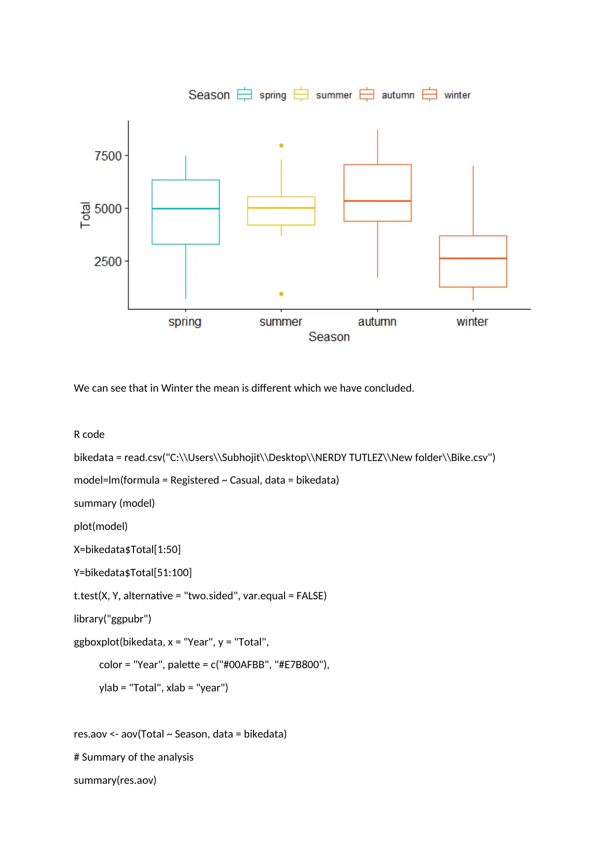
This assignment solution focuses on analyzing bike sharing data using various statistical methods. It includes a simple linear regression analysis examining the relationship between registered and casual users, a two-sample t-test comparing total users in 2011 and 2012, and a one-way ANOVA to assess differences in total users across different seasons. The regression analysis reveals a significant dependence of registered users on casual users. The t-test demonstrates a significant difference in total users between the two years. The ANOVA test indicates that total users vary significantly across different seasons, particularly in winter. The solution provides detailed interpretations of the statistical outputs and includes the R code used for the analysis. Desklib offers a platform where students can find similar solved assignments and past papers for their academic needs.

1)
We have taken the Registered user as the dependent variable and Casual users as the independent
variable.
Now when we are plotting the simple linear regression then we are taking the hypothesis that
H0: The coefficients are not significant in other words we can say that Registered user does not
depends on the Casual users. So the betas are insignificant
H1: The coefficients are significant which means the registered user are dependent on the Casual
users. The betas are significant
Call:
lm(formula = Registered ~ Casual, data = bikedata)
Residuals:
Min 1Q Median 3Q Max
-2280.1 -537.1 -138.7 488.7 1799.2
Coefficients:
Estimate Std. Error t value Pr(>|t|)
(Intercept) 1.027e+03 1.539e+02 6.673 1.5e-09 ***
Casual 1.329e+00 9.458e-02 14.054 < 2e-16 ***
---
Signif. codes: 0 ‘***’ 0.001 ‘**’ 0.01 ‘*’ 0.05 ‘.’ 0.1 ‘ ’ 1
Residual standard error: 780 on 98 degrees of freedom
Multiple R-squared: 0.6684, Adjusted R-squared: 0.665
F-statistic: 197.5 on 1 and 98 DF, p-value: < 2.2e-16
As we can see the p values are much less than 0.05 so both the intercept and the beta are
significant which means registered users is dependent on the casual users.
The different plots which we obtained are

2)
We can use two sample t test to compare the Total users in year 2011 and year 2012.
Null Hypothesis: Means are equal for both year 2011 and year 2012
Alternate Hypothesis: Means are not equal for year 2011 nad year 2012

If we do the two sample t test we get the following output
Welch Two Sample t-test
data: X and Y
t = -6.4188, df = 94.706, p-value = 5.419e-09
alternative hypothesis: true difference in means is not equal to 0
95 percent confidence interval:
-2949.427 -1555.933
sample estimates:
mean of x mean of y
3167.68 5420.36
From the following test we can see that means are not equal to zero and they are different. So the
Total users in year 2011 and year 2012 are different.
We can confirm it from the box plots also the means are at different level.
3)
The four season can be calculated with the help of 1 way ANOVA
In 1 way ANOVA we take the Total as the response variable and the Season as the independent
variable and the hypothesis we take are
H0: The Total users in al the season are same

H1: The total users in all the seasons are different.
When we are applying 1 way ANOVA we get the following results
summary(res.aov)
Df Sum Sq Mean Sq F value Pr(>F)
Season 3 130030562 43343521 13.94 1.29e-07 ***
Residuals 96 298586044 3110271
---
Signif. codes: 0 ‘***’ 0.001 ‘**’ 0.01 ‘*’ 0.05 ‘.’ 0.1 ‘ ’ 1
>
From the analysis we can see that F value is more than the critical so the emans are not same
throughout all the season
Tukey multiple pairwise-comparisons
As the ANOVA test is significant, we can compute Tukey HSD (Tukey Honest Significant Differences,
R function: TukeyHSD()) for performing multiple pairwise-comparison between the means of groups.
The function TukeyHD() takes the fitted ANOVA as an argument.
This test is carrid out to check which two seasons differ.
Tukey multiple comparisons of means
95% family-wise confidence level
Fit: aov(formula = Total ~ Season, data = bikedata)
$`Season`
diff lwr upr p adj
spring-autumn -1013.0385 -2365.9149 339.8379 0.2113316
summer-autumn -478.4385 -1849.8972 893.0203 0.7984361
winter-autumn -2771.4930 -3980.6644 -1562.3216 0.0000002
summer-spring 534.6000 -906.0975 1975.2975 0.7666729
winter-spring -1758.4545 -3045.6242 -471.2849 0.0030745
winter-summer -2293.0545 -3599.7413 -986.3678 0.0000789
from this we can see that winter – summer, winter – spring and winter – autumn are significant.
So the means vary across this season for the total users. So winter makes all the difference in the
mean
If we draw the box plots

We can see that in Winter the mean is different which we have concluded.
R code
bikedata = read.csv("C:\\Users\\Subhojit\\Desktop\\NERDY TUTLEZ\\New folder\\Bike.csv")
model=lm(formula = Registered ~ Casual, data = bikedata)
summary (model)
plot(model)
X=bikedata$Total[1:50]
Y=bikedata$Total[51:100]
t.test(X, Y, alternative = "two.sided", var.equal = FALSE)
library("ggpubr")
ggboxplot(bikedata, x = "Year", y = "Total",
color = "Year", palette = c("#00AFBB", "#E7B800"),
ylab = "Total", xlab = "year")
res.aov <- aov(Total ~ Season, data = bikedata)
# Summary of the analysis
summary(res.aov)

TukeyHSD(res.aov)
ggboxplot(bikedata, x = "Season", y = "Total",
color = "Season", palette = c("#00AFBB", "#E7B800", "#FC4E07", "#FC4E08"),
order = c("spring", "summer", "autumn","winter"),
ylab = "Total", xlab = "Season")