UOW STAT201 Assignment 4: Solutions for Random Variables & Estimation

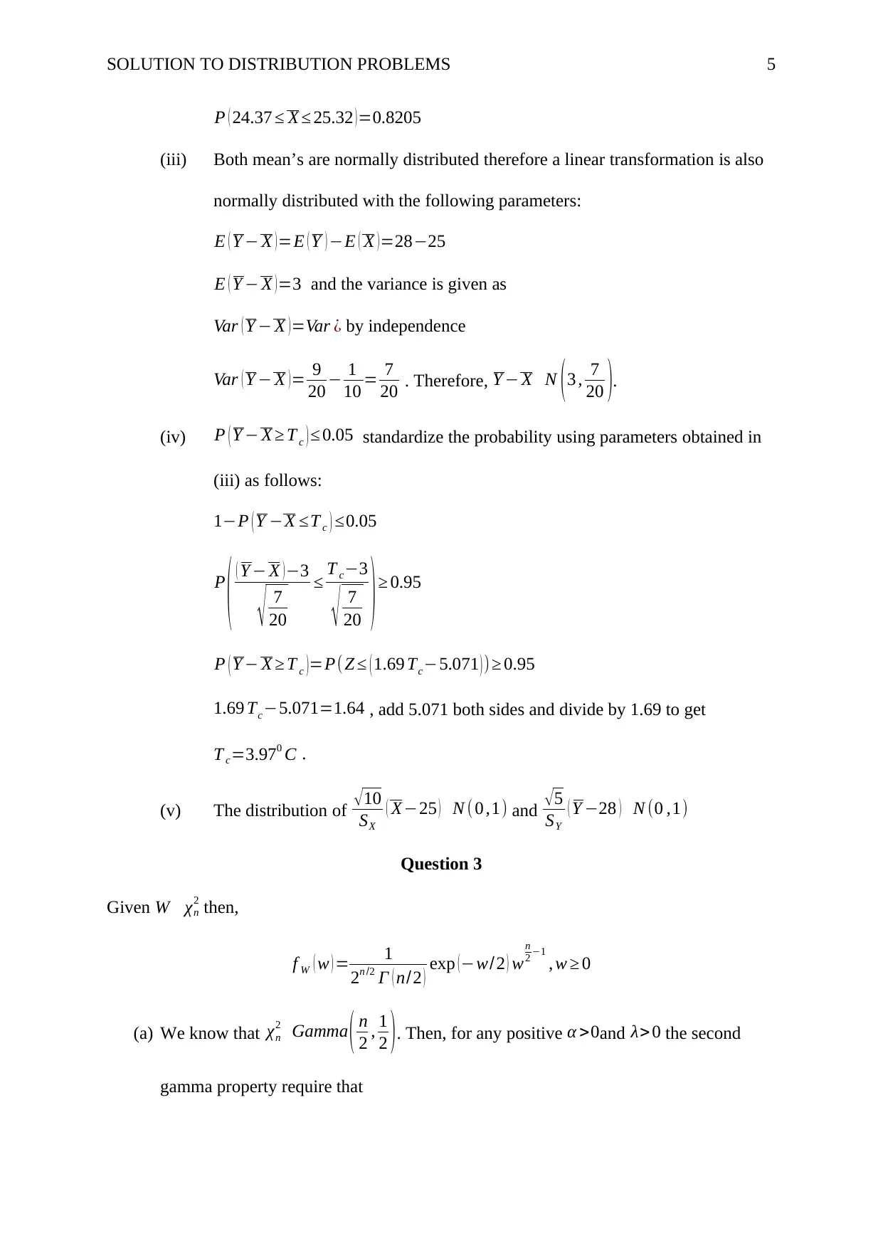
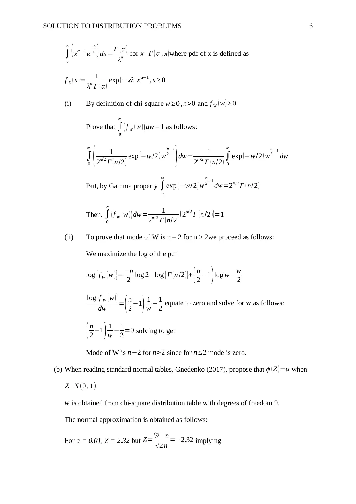
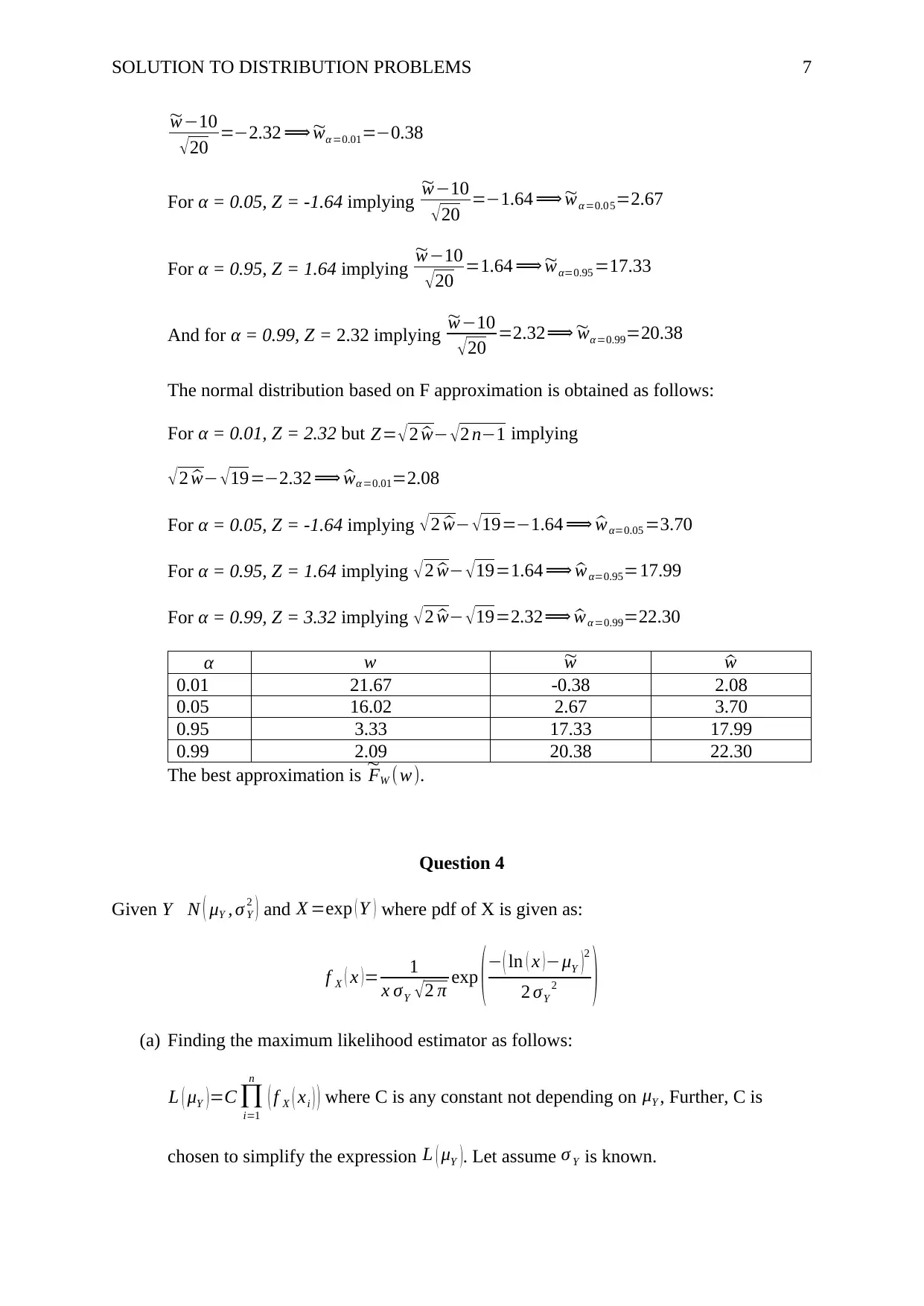
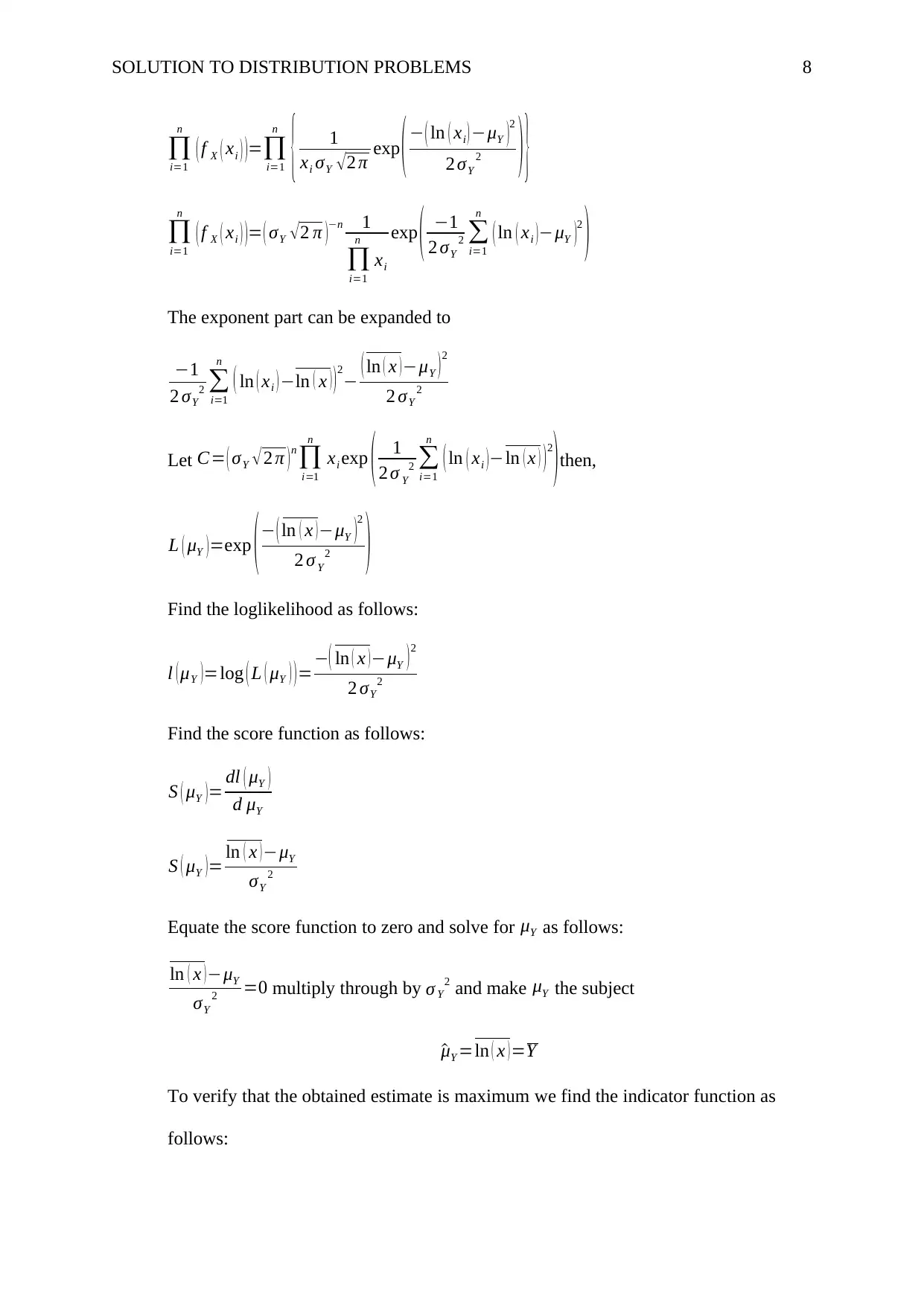
This document presents a comprehensive solution to STAT201 Assignment 4, focusing on distribution problems, random variables, and estimation techniques. The solution addresses several key questions, including calculations related to normal distributions, linear combinations of random variables, and chi-square distributions. It also involves graphical analysis of distributions, and the application of the maximum likelihood estimator (MLE) and the method of moments. The solution includes detailed steps, derivations, and the use of R-code to analyze and visualize the relative efficiency of the MLE compared to the method of moments. The document provides thorough explanations and calculations, making it a valuable resource for students studying statistics and probability. The assignment also covers topics like confidence intervals and the application of the gamma property.

Running head: SOLUTION TO DISTRIBUTION PROBLEMS 1
Solutions to Normal Distribution Problems
Name
Institution

SOLUTION TO DISTRIBUTION PROBLEMS 2
Solutions to Normal Distribution Problems
Question 1
Given X1 , … , X4 N (2 , 3) and Y 1 , … ,Y 4 N (−1, 1).
(a) The distributions are obtained as follows:
According to Fisz and Bartoszyński (2018 if X N ( μ , σ2 ) and X is the sample mean
then X N ( μ , σ2
n ) where n is the sample size.
(i) X +3. This is a linear combination of x’s, therefore,
X N (2 , 3
4 ). Then, the expectation of X +3 is given as follows:
E ( X +3 )=E ( X ) + E ( 3 ) =2+3
E ( X +3 )=5 . Further, the variance of X +3 is given as follows:
Var ( X +3 ) =E ( X +3−E( X + 3) ) 2
Var ( X +3 ) =E ( X +3 ) 2=E ( X2 +6 X + 9)
Var ( X +3 ) =E ( X2 ) +6 E ( X ) +E ( 9 ) =E ( X2 )+ 6 ( 2 ) +9
Var ( X +3 ) =E ( X2 ) +21
But E ( X 2 ) =Var ( X ) + ( E( X ) )2= 3
4 +4=4.75
Then, Var ( X +3 ) =4.75+21=25.75. Therefore,
X +3 N (5 , 25.75).
(ii) X and Y are independent hence the distribution of linear transformation is also
normal. Given, Y 1 N (−1 ,1).
The expectation of 2 X +Y 1 is given as follows:
E ( 2 X +Y 1 ) =2 E ( X )+E ( Y 1 )=2 ( 2 ) +−1
E ( 2 X +Y 1 ) =3 . Further, the variance of 2 X +Y 1 is given as follows:

SOLUTION TO DISTRIBUTION PROBLEMS 3
Var ( 2 X +Y 1 )=4 Var ( X)+Var (Y ¿ ¿1) ¿ by independence.
Var ( 2 X +Y 1 )=4 ( 3
4 )+1
Var ( 2 X +Y 1 ) =4
Therefore,
( 2 X +Y 1 ) N (3 , 4).
According to X N ( μ , σ2 ) then X−μ
σ N (0 , 1) also ( X −μ
σ )2
χ(1)
2 . Further,
∑
i=1
n
( X−μ
σ )2
χ(n)
2 .
With this knowledge the distribution of ( X1−2
√3 )2
+ ( Y 1+1 ) 2.
( X1−2
√ 3 )
2
χ(1)
2 and ( Y 1 +1 )2 χ(1)
2 . Then,
( X1−2
√3 )2
+ ( Y 1+1 ) 2 χ(2)
2 sum of two chi-square distributions.
(iii) We know that χ(u)
2
χ(v )
2 Fu , v.
Now,SX
2 =
∑
i=1
4
( Xi−2 )2
3
SX
2 =∑
i=1
4
( Xi−2
3 )
2
χ(4 )
2
Similarly, SY
2 =
∑
i=1
6
( Y i +1 )2
5
5 SY
2 =∑
i=1
6
( Y i +1 )2 χ(6 )
2
Therefore,

SOLUTION TO DISTRIBUTION PROBLEMS 4
SX
2
5 SY
2 = χ(4)
2
χ(6 )
2 Fu ,v
(b) From (iv) 5 SY
2 χ(6)
2 , then mean of 5 SY
2 =6 and variance 5 SY
2 =12.
Question 2
(a) The plots are symmetric about a point an indication that the two distributions are
normally distributed. From figure 1 the centre of the density function for f X ( x ) is 25
implying μx=250 C. Further, examining the graph approximately 68% of the data lie
between 240 Cand 260 C implying σ X
2 =10 C. Similarly, from figure 1 the centre of the
density function for f Y ( y) is 25 implying μx=280 C. And further examination of the
graph approximately 68% of the data lie between 26. 250 Cand 30. 250 C implying
σ X
2 =2. 2 50 C.
(b) Sample size for X is 10 and for Y is 5. Also, X N (25 , 1) implying X N (25 , 1
10 ).
Similarly, Y N (28 , 2.25) implying X N (25 , 9
20 ).
(i) We know that if X N ( μ , σ2 ) then Z=( X −μ
σ ) N (0 , 1), similarly, if
X N (μ , σ2
n ) then Z=( √ n ( X −μ )
σ ) N (0 , 1).
With the knowledge above √ 10 ( X−25 ) N (0 ,1) similarly,
√ 10
3 ( Y −28 ) N (0 ,1).
(ii) The probability is defined as follows:
P ( 24.37 ≤ X ≤ 25.32 ) standardize the probability
P ( 24.37 ≤ X ≤ 25.32 )=P ( √10 ( 24.37−25 ) ≤ Z ≤ √10 ( 25.32−25 ) )
P ( 24.37 ≤ X ≤ 25.32 )=P(−1.99≤ Z ≤1.01)
P ( 24.37 ≤ X ≤ 25.32 )=ϕ ( 1.01 )−ϕ (−1.99 ) =0.8438−0.0233

SOLUTION TO DISTRIBUTION PROBLEMS 5
P ( 24.37 ≤ X ≤ 25.32 )=0.8205
(iii) Both mean’s are normally distributed therefore a linear transformation is also
normally distributed with the following parameters:
E ( Y − X )=E ( Y ) −E ( X )=28−25
E ( Y − X )=3 and the variance is given as
Var ( Y − X )=Var ¿ by independence
Var ( Y − X )= 9
20 − 1
10 = 7
20 . Therefore, Y − X N (3 , 7
20 ).
(iv) P ( Y − X ≥ T c ) ≤ 0.05 standardize the probability using parameters obtained in
(iii) as follows:
1−P ( Y −X ≤T c ) ≤0.05
P
( ( Y − X )−3
√ 7
20
≤ T c−3
√ 7
20 )≥ 0.95
P ( Y − X ≥ T c )=P(Z ≤ ( 1.69 Tc−5.071 ) ) ≥ 0.95
1.69 Tc−5.071=1.64 , add 5.071 both sides and divide by 1.69 to get
T c=3.970 C .
(v) The distribution of √10
SX
( X−25 ) N (0 ,1) and √ 5
SY
( Y −28 ) N (0 ,1)
Question 3
Given W χn
2 then,
f W ( w ) = 1
2n /2 Γ ( n/2 ) exp (−w/2 ) w
n
2 −1
, w ≥ 0
(a) We know that χn
2 Gamma ( n
2 , 1
2 ). Then, for any positive α >0and λ> 0 the second
gamma property require that

SOLUTION TO DISTRIBUTION PROBLEMS 6
∫
0
∞
(xα−1 e
−x
λ ) dx= Γ ( α )
λα for x Γ ( α , λ )where pdf of x is defined as
f X ( x ) = 1
λα Γ ( α ) exp ( −xλ ) xα−1 , x ≥ 0
(i) By definition of chi-square w ≥ 0 , n>0 and f W ( w ) ≥ 0
Prove that ∫
0
∞
( f W ( w ) ) dw=1 as follows:
∫
0
∞
( 1
2n/ 2 Γ ( n /2 ) exp (−w /2 ) w
n
2 −1
)dw= 1
2n /2 Γ ( n/2 ) ∫
0
∞
exp (−w/2 ) w
n
2 −1
dw
But, by Gamma property ∫
0
∞
exp ( −w/2 ) w
n
2 −1
dw=2n /2 Γ ( n/ 2 )
Then, ∫
0
∞
( f W ( w ) ) dw= 1
2n / 2 Γ ( n/ 2 ) ( 2n/ 2 Γ ( n /2 ) ) =1
(ii) To prove that mode of W is n – 2 for n > 2we proceed as follows:
We maximize the log of the pdf
log { f W ( w ) }=−n
2 log 2−log { Γ ( n /2 ) }+ ( n
2 −1 )log w− w
2
log {f W ( w ) }
dw = ( n
2 −1) 1
w − 1
2 equate to zero and solve for w as follows:
( n
2 −1 ) 1
w −1
2 =0 solving to get
Mode of W is n−2 for n>2 since for n ≤ 2 mode is zero.
(b) When reading standard normal tables, Gnedenko (2017), propose that ϕ ( Z ) =α when
Z N (0 , 1).
w is obtained from chi-square distribution table with degrees of freedom 9.
The normal approximation is obtained as follows:
For α = 0.01, Z = 2.32 but Z= ~w−n
√2 n =−2.32 implying

SOLUTION TO DISTRIBUTION PROBLEMS 7
~w−10
√20 =−2.32 ⟹ ~wα=0.01=−0.38
For α = 0.05, Z = -1.64 implying
~w−10
√ 20 =−1.64 ⟹ ~wα=0.05=2.67
For α = 0.95, Z = 1.64 implying
~w−10
√20 =1.64 ⟹ ~wα=0.95 =17.33
And for α = 0.99, Z = 2.32 implying
~w−10
√ 20 =2.32⟹ ~wα=0.99=20.38
The normal distribution based on F approximation is obtained as follows:
For α = 0.01, Z = 2.32 but Z= √ 2 ^w− √ 2 n−1 implying
√2 ^w− √19=−2.32 ⟹ ^wα=0.01=2.08
For α = 0.05, Z = -1.64 implying √ 2 ^w− √ 19=−1.64 ⟹ ^wα=0.05 =3.70
For α = 0.95, Z = 1.64 implying √ 2 ^w− √ 19=1.64 ⟹ ^wα=0.95=17.99
For α = 0.99, Z = 3.32 implying √ 2 ^w− √ 19=2.32⟹ ^wα =0.99=22.30
α w ~w ^w
0.01 21.67 -0.38 2.08
0.05 16.02 2.67 3.70
0.95 3.33 17.33 17.99
0.99 2.09 20.38 22.30
The best approximation is ~
FW (w).
Question 4
Given Y N ( μY , σ Y
2 ) and X =exp ( Y ) where pdf of X is given as:
f X ( x ) = 1
x σY √ 2 π exp ( − ( ln ( x ) −μY )
2
2 σY
2 )
(a) Finding the maximum likelihood estimator as follows:
L ( μY )=C ∏
i=1
n
( f X ( xi ) ) where C is any constant not depending on μY , Further, C is
chosen to simplify the expression L ( μY ). Let assume σ Y is known.

SOLUTION TO DISTRIBUTION PROBLEMS 8
∏
i=1
n
( f X ( xi ) )=∏
i=1
n
{ 1
xi σY √2 π exp (− ( ln ( xi ) −μY )2
2 σY
2 ) }
∏
i=1
n
( f X ( xi ) )= ( σY √2 π )−n 1
∏
i=1
n
xi
exp ( −1
2 σY
2 ∑
i=1
n
( ln ( xi )−μY )2
)
The exponent part can be expanded to
−1
2 σY
2 ∑
i=1
n
( ln ( xi )−ln ( x ) )2
− ( ln ( x )−μY )2
2 σY
2
Let C= ( σY √ 2 π ) n
∏
i=1
n
xi exp ( 1
2 σ Y
2 ∑
i=1
n
( ln ( xi )−ln ( x ) ) 2
)then,
L ( μY )=exp (− ( ln ( x )−μY )2
2 σ Y
2 )
Find the loglikelihood as follows:
l ( μY )=log ( L ( μY ) )=−( ln ( x )−μY )2
2 σY
2
Find the score function as follows:
S ( μY )= dl ( μY )
d μY
S ( μY )= ln ( x )−μY
σY
2
Equate the score function to zero and solve for μY as follows:
ln ( x )−μY
σY
2 =0 multiply through by σ Y
2 and make μY the subject
^μY =ln ( x )=Y
To verify that the obtained estimate is maximum we find the indicator function as
follows:

SOLUTION TO DISTRIBUTION PROBLEMS 9
I ( μY ) = d S ( μY )
d μY
I ( μY ) =−1
σY
2 this function is negative for all σ Y
2. Hence, the estimate is maximum.
(b) The estimate ^μY is unbiased if E ( ^μY )=μY
Now, E ( ^μY )=E ( ln ( x ) )=E (Y )
Given Y N ( μY , σ Y
2 ) implies Y N (μY , σY
2
n ). Hence, E ( ^μY )=μY
The estimator is unbiased. The variance is given as
Var ( ^μY )=Var ( ln ( x ) )=Var (Y )= σY
2
n the estimate is consistent since as n tend to infinity
the variance approach σ Y
2 .
(c) Given α =0.05, 95% CI is ^μY ± 1, and σ Y
2 =2.
We know that 95% CI is given by the formula is ^μY ±
σY Z α
2
√ n
. But we can find
Z α
2
=Z0.025=1.96 and σ Y = √ 2=1.414
Now,
σY Z α
2
√n =1⟹ 1.414 (1.96 )
√n =1 Thus, n=7.6 ≈ 8.
Therefore, the researcher needs to collect 8 data points to obtain the 95% CI.
(d) Find the expectation as follows:
E [ exp ( ^μY +σY
2 /2 ) ] =exp ( E( ^μY )+σY
2 /2 ) =exp ( μY +σY
2 /2 ) but if n = 1 the variance does
not exist hence biased at that point.

SOLUTION TO DISTRIBUTION PROBLEMS 10
Question 5
Given
f X ( x|θ )= {4 x3 /θ4 0≤ x ≤ θ
0 Otherwise
(a) The sample is dependent on the parameter hence we must use Indicator function
L ( θ ) =C ∏
i=1
n
( f X ( xi|θ ) ) where C is any constant not depending on θ. Further, C is
chosen to simplify the expression L ( θ ).
∏
i=1
n
( f X ( xi|θ ) ) =∏
i=1
n
{ 4 xi
3
θ4 I θ (xi) }
∏
i=1
n
{ 4 xi
3
θ4 I θ ( xi) }=
4 ∏
i=1
n
xi
3
θ4 ∏
i=1
n
I θ (xi)
Let C= 1
4 ∏
i=1
n
xi
3 then,
L ( θ ) = 1
θ4 ∏
i=1
n
I θ ( xi)
Find the loglikelihood as follows:
l ( θ )=log ( L ( θ ) ) =−4 ln θ+ln (∏
i=1
n
Iθ ( xi) )
Find the score function as follows:
S ( θ ) = dl ( θ )
d θ
S ( θ )=−1
θ4 + 1
∏
i=1
n
Iθ ( xi )

SOLUTION TO DISTRIBUTION PROBLEMS 11
Equate the score function to zero and solve for θ as follow:
−1
θ4 + 1
∏
i=1
n
I θ ( xi)
=0
^θ=∏
i=1
n
¿ ¿ Where X(n) is the order statistic?
(b) The method of moments involves finding the first sample mean and equation to
population mean.
E ( X ) =∫
0
θ
x ( 4 x3
θ4 )dx=∫
0
θ
( 4 x4
θ4 )dx= [ 4 x5
5 θ4 ] x=θ
x=0
E ( X ) = 4 θ5
5 θ4 = 4 θ
5
Equate to sample mean
4 θ
5 = X ⟹ ~
θ= 5 X
4
(c) Relative efficiency is obtained as
R ( ^θ
~
θ )=Var ( ^θ)
Var ¿ ¿
Var ( ^θ ) = n
( n+ 1 )2 and Var ¿
But, Var ( X )= 1
n2 ∑
i=1
n
Var ( X ) where Var ( X )=E ( X2 )−E ( X )
E ( X2 ) =∫
0
θ
x2
( 4 x3
θ4 )dx=∫
0
θ
( 4 x5
θ4 )dx =
[ x6
3 θ4 ]x =θ
x =0
E ( X2 ) = θ6
3 θ4 = θ2
3
Then, Var ( X ) = θ2
3 − 4 θ
5 =5 θ2 −12θ
1 5
Var ( X )= 1
n2 ∑
i=1
n
( 5 θ2−12 θ
15 )= 1
n2 ( 5 θ2−12 θ
15 )n

SOLUTION TO DISTRIBUTION PROBLEMS 12
Var ¿
R ( ^θ
~
θ )=Var ( ^θ)
Var ¿ ¿
R ( θ )= 4 (5)n−1 n
( n+1 )2 ( 5 θ2−12 θ )n for n ≥ 1
(d) Let θ=0.5
The R-codes is as follows:
## Define the value of θ used
Theta <- 0.5
## Define the function
Relative.efficiency <- function (n) {(4*5^(n-1)*n)/(((n+1)^2)*((5*Theta^2)-
12*Theta)^n)}
## Plot the function
Plot <- plot(Relative.efficiency(1:100), type = "l", col="blue", main = "Figure 1: Plot
of Relative Efficiency", xlab = "Sample size (n)", ylab = "Relative Efficiency")
Plot
### End of Code##
The figure 1 below shows the plots