STAT6003: Regression Analysis & Sydney House Price Determinants
VerifiedAdded on 2023/05/28
|11
|2643
|328
Case Study
AI Summary
This case study provides a comprehensive regression analysis of Sydney house prices using data from 2002-03 to 2016-17. It identifies market price as the dependent variable and Sydney Price Index, annual percentage change, total area, and age of the house as independent variables. Scatter plots are used to visualize the relationships between the variables. A multiple regression model is constructed and refined, with insignificant variables identified through hypothesis testing. The final model's coefficients are interpreted, and the coefficient of determination is evaluated. A re-estimated linear regression model is compared to the original, highlighting the superior fit of the multiple regression model. The document uses tools like Excel and provides insights into statistical literacy for financial decision-making, offering students a valuable resource; similar assignments and past papers are available on Desklib.

STATISTICS
STUDENT ID:
[Pick the date]
STUDENT ID:
[Pick the date]
Paraphrase This Document
Need a fresh take? Get an instant paraphrase of this document with our AI Paraphraser
1) Introduction
The objective of this report is to present a suitable regression model based on the given
variables. There are five quantitative variables that have been provided in the form of market
price, Sydney Price Index, Annual % change, total size in square meter and also age of the
house. The sample size for the data provided is 15 as data has been provided for 15 years.
Considering the given variables, the first task is to identify a suitable model which has one
dependent variable and four independent variables. Since the measurement scale for each of
the variables is a ratio scale with a defined zero coupled with numerical values, it is easier to
include all the given variables in the form of a multiple regression model. With regards to
such model, the suitable dependent variable would be the price of the house while the other
four variables would serve as the independent variables. This seems quite appropriate
considering that price of house must be function of the area and age. Also, it should also be
dependent on the change in the price index and annual change in property prices that is
witnessed in the underlying area. Thus, a multiple regression model would be framed using
these variables and subsequently refined to remove those independent variables which are not
found to be significant.
2) Scatter Plot
The objective here is to obtain the scatter plot with regards to each of the independent
variables and the dependent variable identified for the multiple regression model.
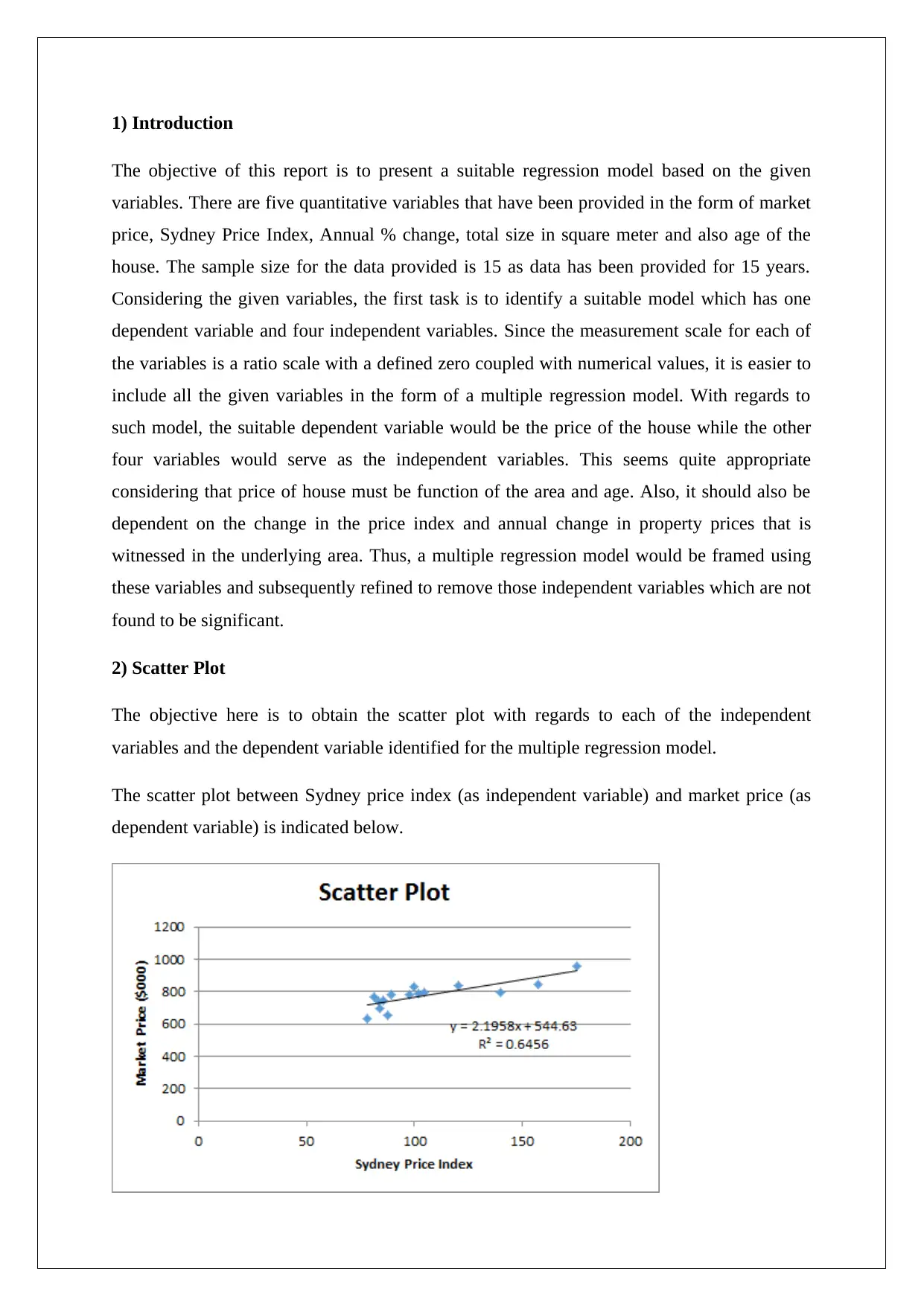
The scatter plot between Sydney price index (as independent variable) and market price (as
dependent variable) is indicated below.
The objective of this report is to present a suitable regression model based on the given
variables. There are five quantitative variables that have been provided in the form of market
price, Sydney Price Index, Annual % change, total size in square meter and also age of the
house. The sample size for the data provided is 15 as data has been provided for 15 years.
Considering the given variables, the first task is to identify a suitable model which has one
dependent variable and four independent variables. Since the measurement scale for each of
the variables is a ratio scale with a defined zero coupled with numerical values, it is easier to
include all the given variables in the form of a multiple regression model. With regards to
such model, the suitable dependent variable would be the price of the house while the other
four variables would serve as the independent variables. This seems quite appropriate
considering that price of house must be function of the area and age. Also, it should also be
dependent on the change in the price index and annual change in property prices that is
witnessed in the underlying area. Thus, a multiple regression model would be framed using
these variables and subsequently refined to remove those independent variables which are not
found to be significant.
2) Scatter Plot
The objective here is to obtain the scatter plot with regards to each of the independent
variables and the dependent variable identified for the multiple regression model.
The scatter plot between Sydney price index (as independent variable) and market price (as
dependent variable) is indicated below.
It is apparent that the best fit line for the above plot is upward slopping which implies that
positive linear relationship tends to exist between the given independent and dependent
variable. Also, considering the low extent of deviation of scatter points from the line of best
fit, it can be concluded that the magnitude of correlation is high with the corresponding
correlation coefficient exceeding 0.8. Thus, the association between the Sydney Price Index
and the market price seems to be significant and positive in nature (Flick, 2015).
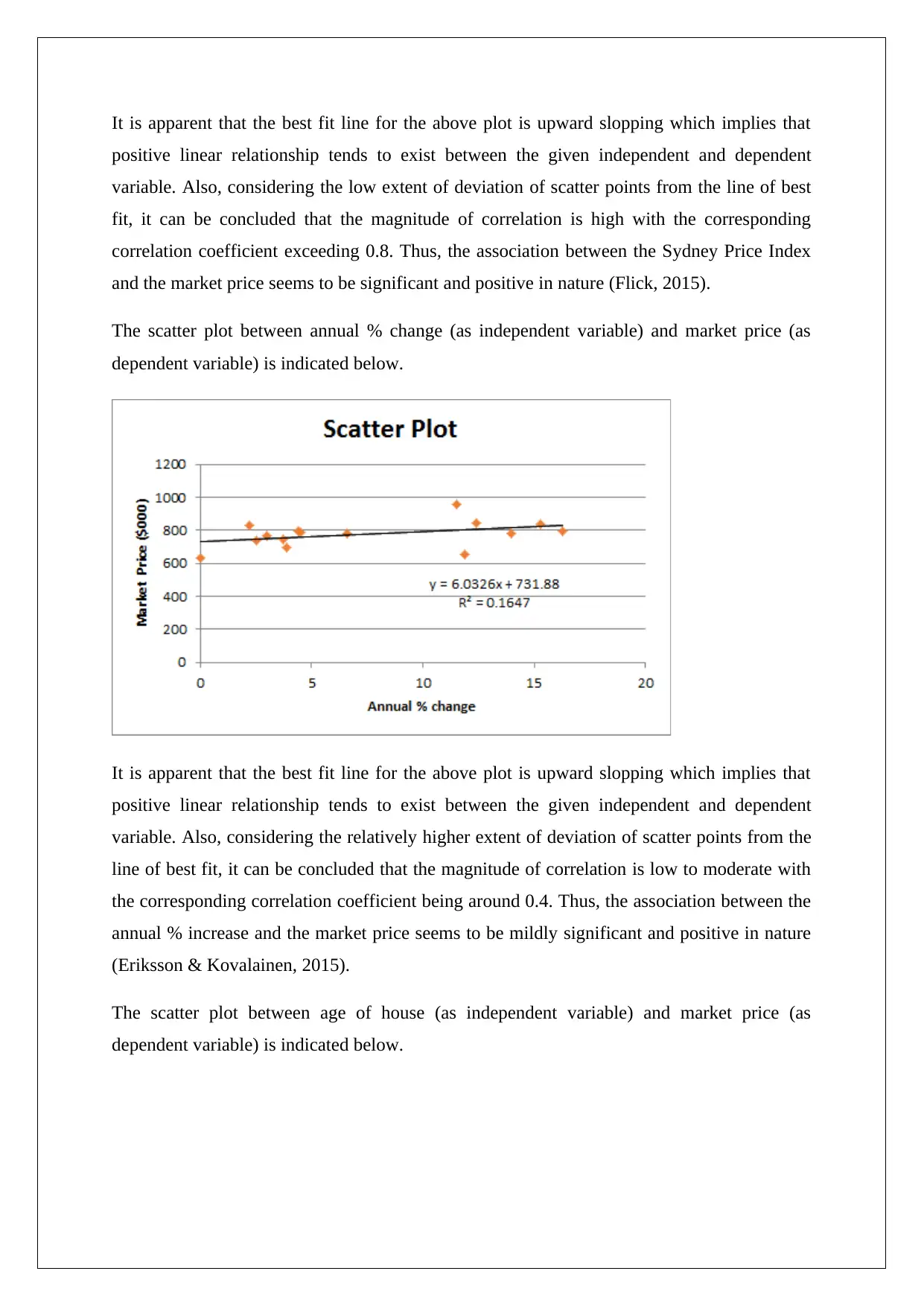
The scatter plot between annual % change (as independent variable) and market price (as
dependent variable) is indicated below.
It is apparent that the best fit line for the above plot is upward slopping which implies that
positive linear relationship tends to exist between the given independent and dependent
variable. Also, considering the relatively higher extent of deviation of scatter points from the
line of best fit, it can be concluded that the magnitude of correlation is low to moderate with
the corresponding correlation coefficient being around 0.4. Thus, the association between the
annual % increase and the market price seems to be mildly significant and positive in nature
(Eriksson & Kovalainen, 2015).
The scatter plot between age of house (as independent variable) and market price (as
dependent variable) is indicated below.
positive linear relationship tends to exist between the given independent and dependent
variable. Also, considering the low extent of deviation of scatter points from the line of best
fit, it can be concluded that the magnitude of correlation is high with the corresponding
correlation coefficient exceeding 0.8. Thus, the association between the Sydney Price Index
and the market price seems to be significant and positive in nature (Flick, 2015).
The scatter plot between annual % change (as independent variable) and market price (as
dependent variable) is indicated below.
It is apparent that the best fit line for the above plot is upward slopping which implies that
positive linear relationship tends to exist between the given independent and dependent
variable. Also, considering the relatively higher extent of deviation of scatter points from the
line of best fit, it can be concluded that the magnitude of correlation is low to moderate with
the corresponding correlation coefficient being around 0.4. Thus, the association between the
annual % increase and the market price seems to be mildly significant and positive in nature
(Eriksson & Kovalainen, 2015).
The scatter plot between age of house (as independent variable) and market price (as
dependent variable) is indicated below.
⊘ This is a preview!⊘
Do you want full access?
Subscribe today to unlock all pages.
Trusted by 1+ million students worldwide
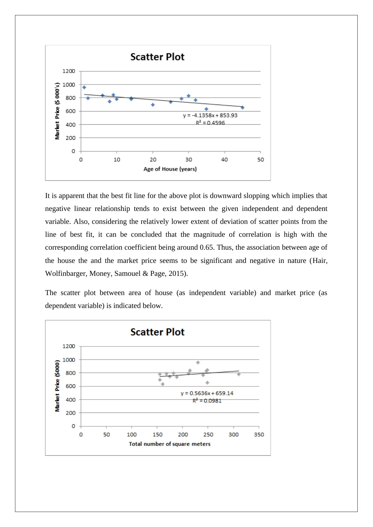
It is apparent that the best fit line for the above plot is downward slopping which implies that
negative linear relationship tends to exist between the given independent and dependent
variable. Also, considering the relatively lower extent of deviation of scatter points from the
line of best fit, it can be concluded that the magnitude of correlation is high with the
corresponding correlation coefficient being around 0.65. Thus, the association between age of
the house the and the market price seems to be significant and negative in nature (Hair,
Wolfinbarger, Money, Samouel & Page, 2015).
The scatter plot between area of house (as independent variable) and market price (as
dependent variable) is indicated below.
Paraphrase This Document
Need a fresh take? Get an instant paraphrase of this document with our AI Paraphraser
It is apparent that the best fit line for the above plot is upward slopping which implies that
positive linear relationship tends to exist between the given independent and dependent
variable. Also, considering the relatively high extent of deviation of scatter points from the
line of best fit, it can be concluded that the magnitude of correlation is low with the
corresponding correlation coefficient being around 0.3. Thus, the association between the
area of the house and the market price seems to be mildly significant and positive in nature
(Hillier, 2016).
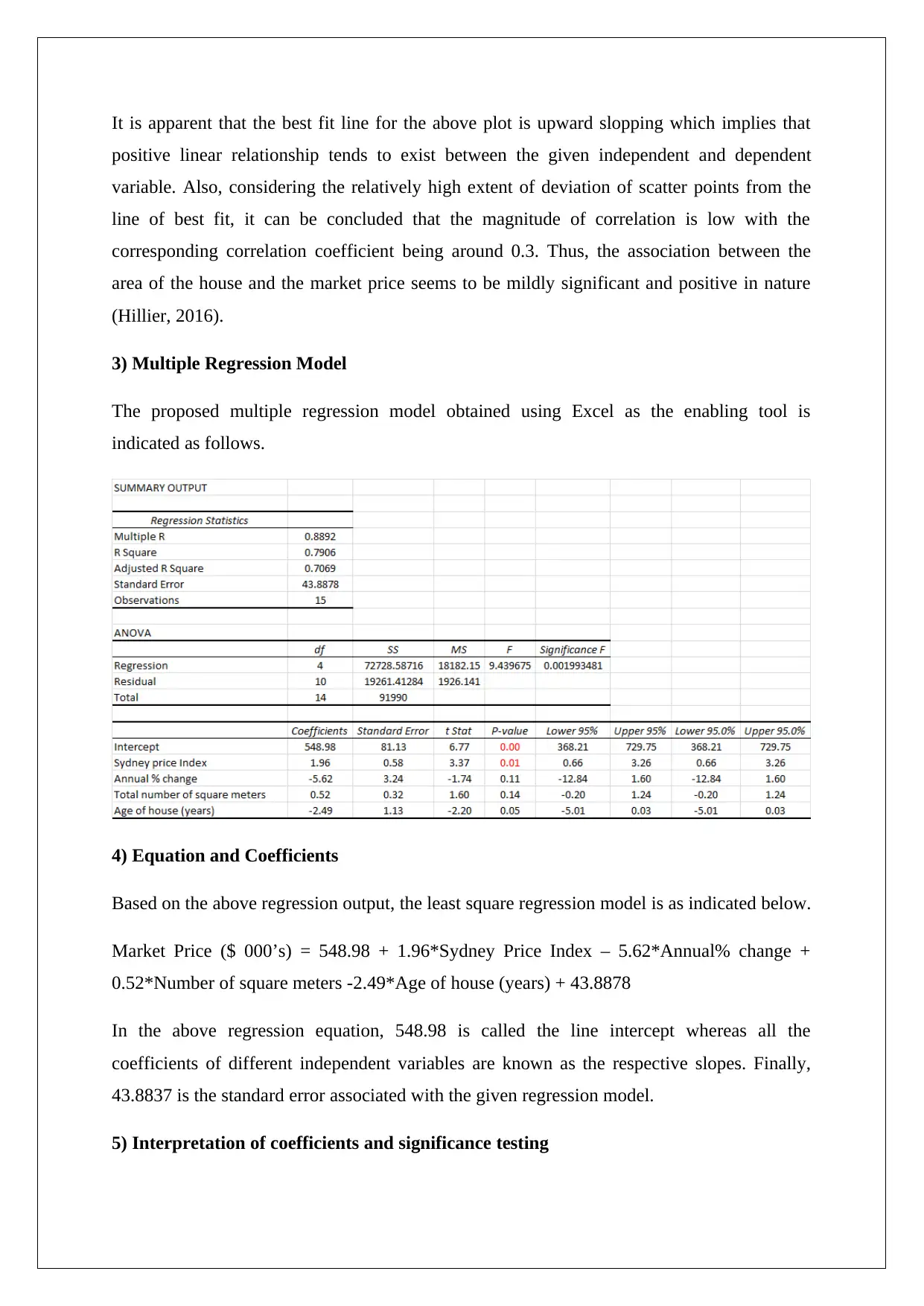
3) Multiple Regression Model
The proposed multiple regression model obtained using Excel as the enabling tool is
indicated as follows.
4) Equation and Coefficients
Based on the above regression output, the least square regression model is as indicated below.
Market Price ($ 000’s) = 548.98 + 1.96*Sydney Price Index – 5.62*Annual% change +
0.52*Number of square meters -2.49*Age of house (years) + 43.8878
In the above regression equation, 548.98 is called the line intercept whereas all the
coefficients of different independent variables are known as the respective slopes. Finally,
43.8837 is the standard error associated with the given regression model.
5) Interpretation of coefficients and significance testing
positive linear relationship tends to exist between the given independent and dependent
variable. Also, considering the relatively high extent of deviation of scatter points from the
line of best fit, it can be concluded that the magnitude of correlation is low with the
corresponding correlation coefficient being around 0.3. Thus, the association between the
area of the house and the market price seems to be mildly significant and positive in nature
(Hillier, 2016).
3) Multiple Regression Model
The proposed multiple regression model obtained using Excel as the enabling tool is
indicated as follows.
4) Equation and Coefficients
Based on the above regression output, the least square regression model is as indicated below.
Market Price ($ 000’s) = 548.98 + 1.96*Sydney Price Index – 5.62*Annual% change +
0.52*Number of square meters -2.49*Age of house (years) + 43.8878
In the above regression equation, 548.98 is called the line intercept whereas all the
coefficients of different independent variables are known as the respective slopes. Finally,
43.8837 is the standard error associated with the given regression model.
5) Interpretation of coefficients and significance testing

The interpretation of the various coefficients is given below.
Intercept – This value highlights the market price of house when all the independent variables
are zero. Clearly, this is not of any significance or practical utility in the given linear model.
Slope coefficient (Sydney Price Index) – The slope coefficient of this independent variable is
1.96. This implies that a unit change in the Sydney Price Index would alter the market price
of the house by $ 1,960. The movement of the market price of the house would be in the
same direction as the movement in the independent variable (Fehr & Grossman, 2013).
Slope coefficient (Annual % change) - The slope coefficient of this independent variable is -
5.62. This implies that a percentage change in this variable would alter the market price of the
house by $ 5,620. The movement of the market price of the house would be in the opposite
direction as the movement in the independent variable (Medhi, 2016).
Slope coefficient (Number of square metres) - The slope coefficient of this independent
variable is 0.52. This implies that a unit change in the number of square feet would alter the
market price of the house by $520. The movement of the market price of the house would be
in the same direction as the movement in the independent variable.
Slope coefficient (Age of house) - The slope coefficient of this independent variable is -2.49.
This implies that a percentage change in this variable would alter the market price of the
house by $ 2,490. The movement of the market price of the house would be in the opposite
direction as the movement in the independent variable (Hastie, Tibshirani and Friedman,
2014).
The significance of the above coefficients can be determined using the hypothesis test
indicated below.
Sydney Price Index
Null Hypothesis: βSydney Price Index = 0 i.e. the given slope coefficient can be assumed as zero and
therefore is not significant.
Alternative Hypothesis: βSydney Price Index ≠ 0 i.e. the given slope coefficient cannot be assumed as
zero and therefore is significant.
⊘ This is a preview!⊘
Do you want full access?
Subscribe today to unlock all pages.
Trusted by 1+ million students worldwide
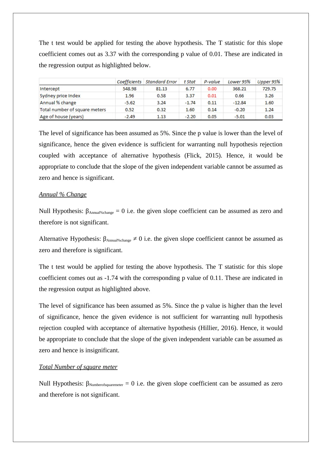
The t test would be applied for testing the above hypothesis. The T statistic for this slope
coefficient comes out as 3.37 with the corresponding p value of 0.01. These are indicated in
the regression output as highlighted below.
The level of significance has been assumed as 5%. Since the p value is lower than the level of
significance, hence the given evidence is sufficient for warranting null hypothesis rejection
coupled with acceptance of alternative hypothesis (Flick, 2015). Hence, it would be
appropriate to conclude that the slope of the given independent variable cannot be assumed as
zero and hence is significant.
Annual % Change
Null Hypothesis: βAnnual%change = 0 i.e. the given slope coefficient can be assumed as zero and
therefore is not significant.
Alternative Hypothesis: βAnnual%change ≠ 0 i.e. the given slope coefficient cannot be assumed as
zero and therefore is significant.
The t test would be applied for testing the above hypothesis. The T statistic for this slope
coefficient comes out as -1.74 with the corresponding p value of 0.11. These are indicated in
the regression output as highlighted above.
The level of significance has been assumed as 5%. Since the p value is higher than the level
of significance, hence the given evidence is not sufficient for warranting null hypothesis
rejection coupled with acceptance of alternative hypothesis (Hillier, 2016). Hence, it would
be appropriate to conclude that the slope of the given independent variable can be assumed as
zero and hence is insignificant.
Total Number of square meter
Null Hypothesis: βNumberofsquaremeter = 0 i.e. the given slope coefficient can be assumed as zero
and therefore is not significant.
Paraphrase This Document
Need a fresh take? Get an instant paraphrase of this document with our AI Paraphraser
Alternative Hypothesis: βNumberofsquaremeter ≠ 0 i.e. the given slope coefficient cannot be assumed
as zero and therefore is significant.
The t test would be applied for testing the above hypothesis. The T statistic for this slope
coefficient comes out as 1.60 with the corresponding p value of 0.14. These are indicated in
the regression output as highlighted above.
The level of significance has been assumed as 5%. Since the p value is higher than the level
of significance, hence the given evidence is not sufficient for warranting null hypothesis
rejection coupled with acceptance of alternative hypothesis (Hair, Wolfinbarger, Money,
Samouel & Page, 2015). Hence, it would be appropriate to conclude that the slope of the
given independent variable can be assumed as zero and hence is insignificant.
Age of House (years)
Null Hypothesis: βAgeofhouse = 0 i.e. the given slope coefficient can be assumed as zero and
therefore is not significant.
Alternative Hypothesis: βAgeofhouse ≠ 0 i.e. the given slope coefficient cannot be assumed as
zero and therefore is significant.
The t test would be applied for testing the above hypothesis. The T statistic for this slope
coefficient comes out as -2.20 with the corresponding p value of 0.52. These are indicated in
the regression output as highlighted above.
The level of significance has been assumed as 5%. Since the p value is higher than the level
of significance, hence the given evidence is not sufficient for warranting null hypothesis
rejection coupled with acceptance of alternative hypothesis (Medhi, 2016). Hence, it would
be appropriate to conclude that the slope of the given independent variable can be assumed as
zero and hence is insignificant.
6) Coefficient of Determination
The coefficient of determination in the given multiple regression model is 0.7906. This
implies that the four independent variables jointly can offer explanation to 79.06% of the
variations observed in the market price of house. Hence, the given model leaves only 20.94%
of the variation in the house price unexplained. Therefore, it can be indicated that the given
regression model presents a good fit (Hastie, Tibshirani & Friedman, 2014).
7) Confidence interval & interpretation
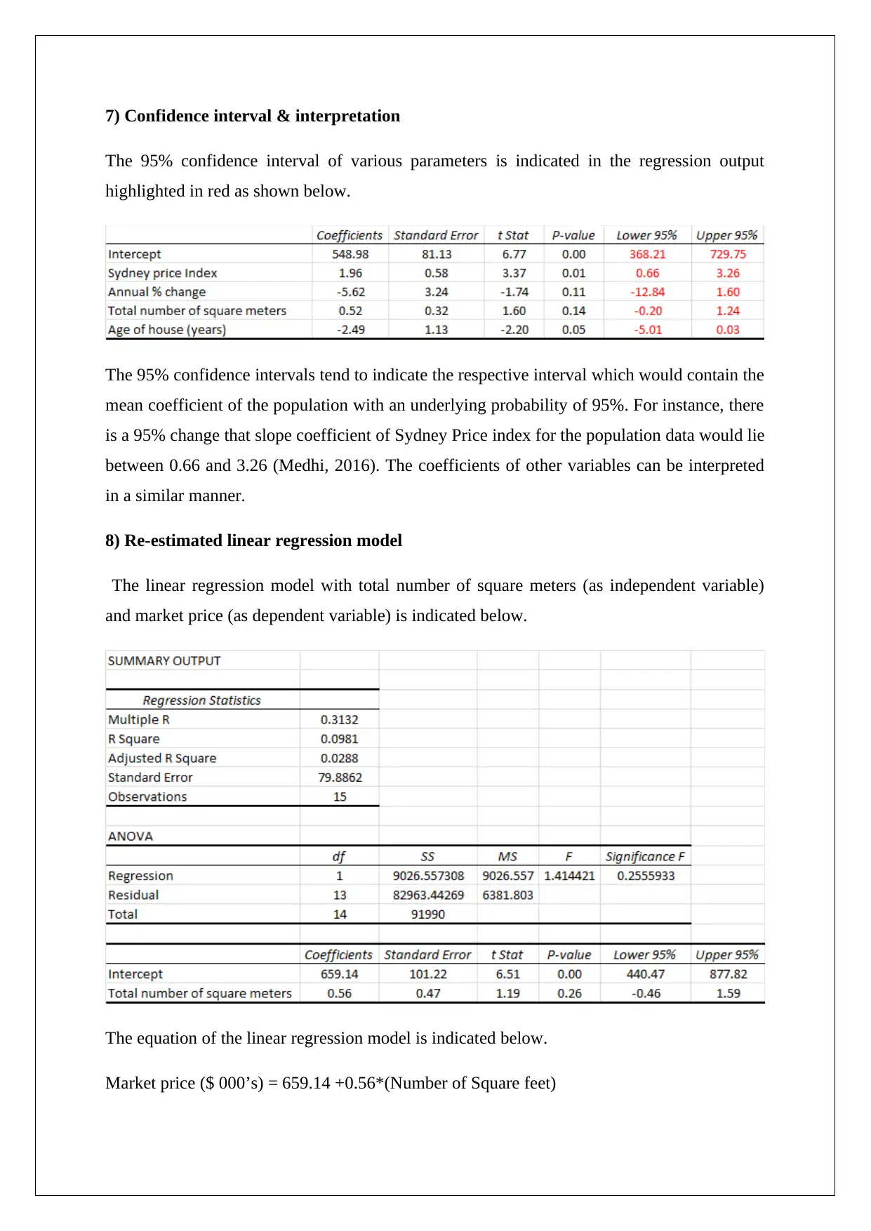
The 95% confidence interval of various parameters is indicated in the regression output
highlighted in red as shown below.
The 95% confidence intervals tend to indicate the respective interval which would contain the
mean coefficient of the population with an underlying probability of 95%. For instance, there
is a 95% change that slope coefficient of Sydney Price index for the population data would lie
between 0.66 and 3.26 (Medhi, 2016). The coefficients of other variables can be interpreted
in a similar manner.
8) Re-estimated linear regression model
The linear regression model with total number of square meters (as independent variable)
and market price (as dependent variable) is indicated below.
The equation of the linear regression model is indicated below.
Market price ($ 000’s) = 659.14 +0.56*(Number of Square feet)
⊘ This is a preview!⊘
Do you want full access?
Subscribe today to unlock all pages.
Trusted by 1+ million students worldwide
9) Comparison of two models
The R2 value for the original multiple regression model was 0.7906 in comparison to the
corresponding value of 0.0981 for the linear regression model. It is apparent that the re-
estimated model (linear regression model) does not represent a good fit as the independent
variable can only offer explanation for about 9.81% of the changes witnessed in the market
price of houses (Hair, Wolfinbarger, Money, Samouel & Page, 2015). Also, focusing on the
relevant t stat and p value of the slope coefficient in the re-estimated model, it is apparent that
the slope coefficient is not significant even if the significance level is assumed to be 10%
(Eriksson & Kovalainen, 2015). Hence, it would be fair to conclude that the original model
was significantly superior to the current model as it had a significantly better fit owing to the
presence of significant independent variables.
10) Estimation of market price of house
Considering that only the building area has been given with no other independent variable,
hence the re-estimated linear regression model would be used in this case. The relevant
equation is indicated below.
Market price ($ 000’s) = 659.14 +0.56*(Number of Square feet)
Number of square feet = 400
Market price ($000’s) = 659.14 +0.56*400 = 884.58
Hence, the market price of the given house should be $ 884,580.
Paraphrase This Document
Need a fresh take? Get an instant paraphrase of this document with our AI Paraphraser
References
Eriksson, P. & Kovalainen, A. (2015) Quantitative methods in business research. 3rd ed.
London: Sage Publications.
Fehr, F. H. & Grossman, G. (2013). An introduction to sets, probability and hypothesis
testing. 3rd ed. Ohio: Heath.
Flick, U. (2015) Introducing research methodology: A beginner's guide to doing a research
project. 4th ed. New York: Sage Publications.
Hair, J. F., Wolfinbarger, M., Money, A. H., Samouel, P., & Page, M. J. (2015) Essentials of
business research methods. 2nd ed. New York: Routledge.
Hastie, T., Tibshirani, R. & Friedman, J. (2014) The Elements of Statistical Learning. 4th
ed. New York: Springer Publications.
Hillier, F. (2016) Introduction to Operations Research. 6th ed. New York: McGraw Hill
Publications.
Medhi, J. (2016) Statistical Methods: An Introductory Text. 4th ed. Sydney: New Age
International.
1 out of 11
Related Documents


Your All-in-One AI-Powered Toolkit for Academic Success.
+13062052269
info@desklib.com
Available 24*7 on WhatsApp / Email
![[object Object]](/_next/static/media/star-bottom.7253800d.svg)
Unlock your academic potential
Copyright © 2020–2026 A2Z Services. All Rights Reserved. Developed and managed by ZUCOL.