Logistic Regression Analysis of Survey Data in Stata - Sleep Study
VerifiedAdded on 2023/04/24
|10
|1769
|101
Homework Assignment
AI Summary
This assignment provides solutions to questions involving logistic regression analysis performed in Stata. The first question explores the impact of gender and faculty on getting at least 7 hours of sleep, analyzing why the odds ratio changes when both variables are included. It assesses the interaction effect between faculty and gender, determining its statistical significance. The second question examines the relationship between quartiles of n-3 fatty acids and smoking habits using conditional logistic regression. It compares a correct model incorporating a grouping variable with an incorrect model that ignores it, highlighting the importance of controlling for confounding variables in case-control studies. Desklib provides access to past papers and solved assignments.
Running head: LOGISTIC REGRESSION IN STATA 1
logistic regression in Stata
institution affiliation
name of student
logistic regression in Stata
institution affiliation
name of student
Paraphrase This Document
Need a fresh take? Get an instant paraphrase of this document with our AI Paraphraser
LOGISTIC REGRESSION IN STATA 2
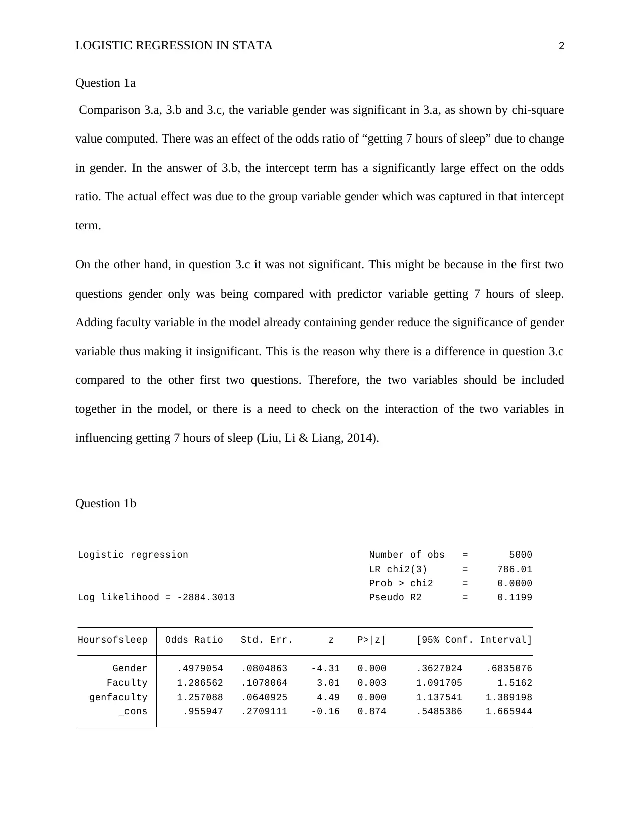
Question 1a
Comparison 3.a, 3.b and 3.c, the variable gender was significant in 3.a, as shown by chi-square
value computed. There was an effect of the odds ratio of “getting 7 hours of sleep” due to change
in gender. In the answer of 3.b, the intercept term has a significantly large effect on the odds
ratio. The actual effect was due to the group variable gender which was captured in that intercept
term.
On the other hand, in question 3.c it was not significant. This might be because in the first two
questions gender only was being compared with predictor variable getting 7 hours of sleep.
Adding faculty variable in the model already containing gender reduce the significance of gender
variable thus making it insignificant. This is the reason why there is a difference in question 3.c
compared to the other first two questions. Therefore, the two variables should be included
together in the model, or there is a need to check on the interaction of the two variables in
influencing getting 7 hours of sleep (Liu, Li & Liang, 2014).
Question 1b
_cons .955947 .2709111 -0.16 0.874 .5485386 1.665944
genfaculty 1.257088 .0640925 4.49 0.000 1.137541 1.389198
Faculty 1.286562 .1078064 3.01 0.003 1.091705 1.5162
Gender .4979054 .0804863 -4.31 0.000 .3627024 .6835076
Hoursofsleep Odds Ratio Std. Err. z P>|z| [95% Conf. Interval]
Log likelihood = -2884.3013 Pseudo R2 = 0.1199
Prob > chi2 = 0.0000
LR chi2(3) = 786.01
Logistic regression Number of obs = 5000
LOGISTIC REGRESSION IN STATA 3
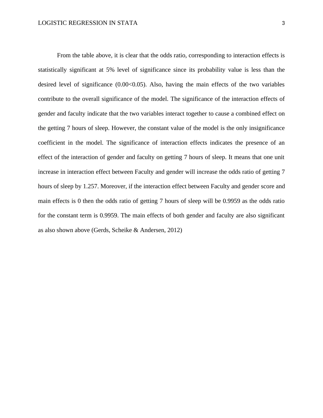
From the table above, it is clear that the odds ratio, corresponding to interaction effects is
statistically significant at 5% level of significance since its probability value is less than the
desired level of significance (0.00<0.05). Also, having the main effects of the two variables
contribute to the overall significance of the model. The significance of the interaction effects of
gender and faculty indicate that the two variables interact together to cause a combined effect on
the getting 7 hours of sleep. However, the constant value of the model is the only insignificance
coefficient in the model. The significance of interaction effects indicates the presence of an
effect of the interaction of gender and faculty on getting 7 hours of sleep. It means that one unit
increase in interaction effect between Faculty and gender will increase the odds ratio of getting 7
hours of sleep by 1.257. Moreover, if the interaction effect between Faculty and gender score and
main effects is 0 then the odds ratio of getting 7 hours of sleep will be 0.9959 as the odds ratio
for the constant term is 0.9959. The main effects of both gender and faculty are also significant
as also shown above (Gerds, Scheike & Andersen, 2012)
⊘ This is a preview!⊘
Do you want full access?
Subscribe today to unlock all pages.
Trusted by 1+ million students worldwide
LOGISTIC REGRESSION IN STATA 4
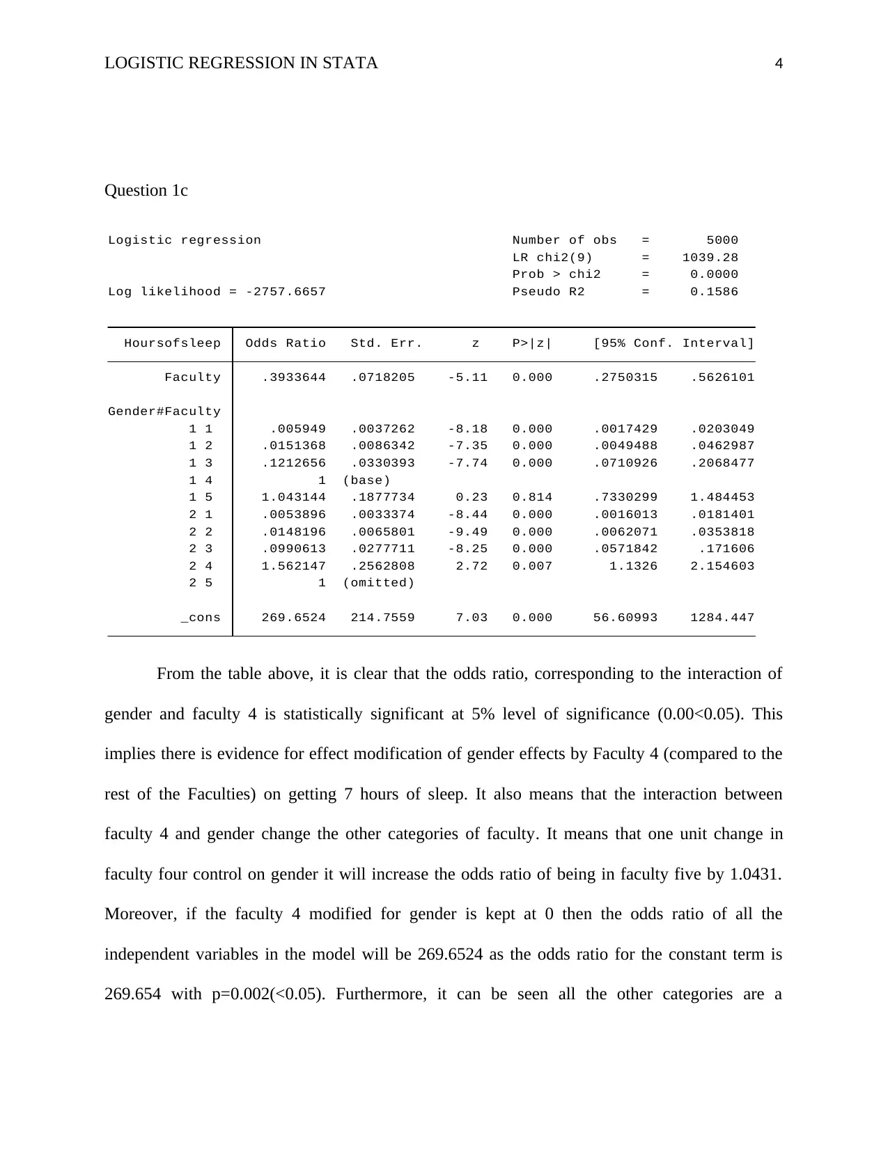
Question 1c
_cons 269.6524 214.7559 7.03 0.000 56.60993 1284.447
2 5 1 (omitted)
2 4 1.562147 .2562808 2.72 0.007 1.1326 2.154603
2 3 .0990613 .0277711 -8.25 0.000 .0571842 .171606
2 2 .0148196 .0065801 -9.49 0.000 .0062071 .0353818
2 1 .0053896 .0033374 -8.44 0.000 .0016013 .0181401
1 5 1.043144 .1877734 0.23 0.814 .7330299 1.484453
1 4 1 (base)
1 3 .1212656 .0330393 -7.74 0.000 .0710926 .2068477
1 2 .0151368 .0086342 -7.35 0.000 .0049488 .0462987
1 1 .005949 .0037262 -8.18 0.000 .0017429 .0203049
Gender#Faculty
Faculty .3933644 .0718205 -5.11 0.000 .2750315 .5626101
Hoursofsleep Odds Ratio Std. Err. z P>|z| [95% Conf. Interval]
Log likelihood = -2757.6657 Pseudo R2 = 0.1586
Prob > chi2 = 0.0000
LR chi2(9) = 1039.28
Logistic regression Number of obs = 5000
From the table above, it is clear that the odds ratio, corresponding to the interaction of
gender and faculty 4 is statistically significant at 5% level of significance (0.00<0.05). This
implies there is evidence for effect modification of gender effects by Faculty 4 (compared to the
rest of the Faculties) on getting 7 hours of sleep. It also means that the interaction between
faculty 4 and gender change the other categories of faculty. It means that one unit change in
faculty four control on gender it will increase the odds ratio of being in faculty five by 1.0431.
Moreover, if the faculty 4 modified for gender is kept at 0 then the odds ratio of all the
independent variables in the model will be 269.6524 as the odds ratio for the constant term is
269.654 with p=0.002(<0.05). Furthermore, it can be seen all the other categories are a
Paraphrase This Document
Need a fresh take? Get an instant paraphrase of this document with our AI Paraphraser
LOGISTIC REGRESSION IN STATA 5
statistically significant reference to faculty four confounded for gender except the fifth faculty
and male.
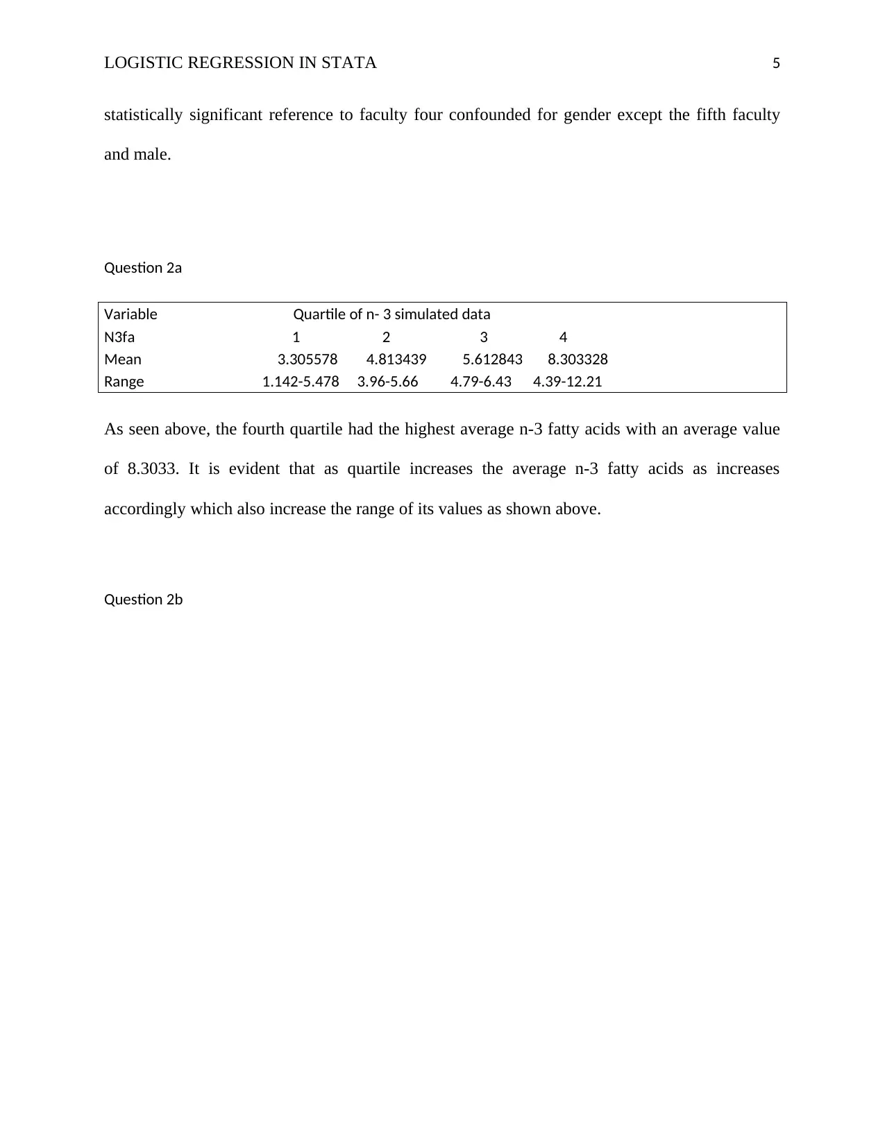
Question 2a
Variable Quartile of n- 3 simulated data
N3fa 1 2 3 4
Mean 3.305578 4.813439 5.612843 8.303328
Range 1.142-5.478 3.96-5.66 4.79-6.43 4.39-12.21
As seen above, the fourth quartile had the highest average n-3 fatty acids with an average value
of 8.3033. It is evident that as quartile increases the average n-3 fatty acids as increases
accordingly which also increase the range of its values as shown above.
Question 2b
statistically significant reference to faculty four confounded for gender except the fifth faculty
and male.
Question 2a
Variable Quartile of n- 3 simulated data
N3fa 1 2 3 4
Mean 3.305578 4.813439 5.612843 8.303328
Range 1.142-5.478 3.96-5.66 4.79-6.43 4.39-12.21
As seen above, the fourth quartile had the highest average n-3 fatty acids with an average value
of 8.3033. It is evident that as quartile increases the average n-3 fatty acids as increases
accordingly which also increase the range of its values as shown above.
Question 2b
LOGISTIC REGRESSION IN STATA 6
.
4 .0157873 .0262181 -2.50 0.012 .0006091 .409174
3 .115105 .1171114 -2.12 0.034 .0156695 .8455378
2 .3271804 .2802103 -1.30 0.192 .0610639 1.753033
n3fa4
n3fa 1.144749 .2559955 0.60 0.546 .738515 1.774438
Casecont Odds Ratio Std. Err. z P>|z| [95% Conf. Interval]
Log likelihood = -92.544007 Pseudo R2 = 0.0896
Prob > chi2 = 0.0011
LR chi2(4) = 18.21
Conditional (fixed-effects) logistic regression Number of obs = 278
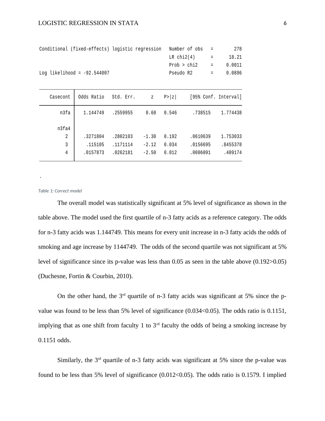
Table 1: Correct model
The overall model was statistically significant at 5% level of significance as shown in the
table above. The model used the first quartile of n-3 fatty acids as a reference category. The odds
for n-3 fatty acids was 1.144749. This means for every unit increase in n-3 fatty acids the odds of
smoking and age increase by 1144749. The odds of the second quartile was not significant at 5%
level of significance since its p-value was less than 0.05 as seen in the table above (0.192>0.05)
(Duchesne, Fortin & Courbin, 2010).
On the other hand, the 3rd quartile of n-3 fatty acids was significant at 5% since the p-
value was found to be less than 5% level of significance (0.034<0.05). The odds ratio is 0.1151,
implying that as one shift from faculty 1 to 3rd faculty the odds of being a smoking increase by
0.1151 odds.
Similarly, the 3rd quartile of n-3 fatty acids was significant at 5% since the p-value was
found to be less than 5% level of significance (0.012<0.05). The odds ratio is 0.1579. I implied
.
4 .0157873 .0262181 -2.50 0.012 .0006091 .409174
3 .115105 .1171114 -2.12 0.034 .0156695 .8455378
2 .3271804 .2802103 -1.30 0.192 .0610639 1.753033
n3fa4
n3fa 1.144749 .2559955 0.60 0.546 .738515 1.774438
Casecont Odds Ratio Std. Err. z P>|z| [95% Conf. Interval]
Log likelihood = -92.544007 Pseudo R2 = 0.0896
Prob > chi2 = 0.0011
LR chi2(4) = 18.21
Conditional (fixed-effects) logistic regression Number of obs = 278
Table 1: Correct model
The overall model was statistically significant at 5% level of significance as shown in the
table above. The model used the first quartile of n-3 fatty acids as a reference category. The odds
for n-3 fatty acids was 1.144749. This means for every unit increase in n-3 fatty acids the odds of
smoking and age increase by 1144749. The odds of the second quartile was not significant at 5%
level of significance since its p-value was less than 0.05 as seen in the table above (0.192>0.05)
(Duchesne, Fortin & Courbin, 2010).
On the other hand, the 3rd quartile of n-3 fatty acids was significant at 5% since the p-
value was found to be less than 5% level of significance (0.034<0.05). The odds ratio is 0.1151,
implying that as one shift from faculty 1 to 3rd faculty the odds of being a smoking increase by
0.1151 odds.
Similarly, the 3rd quartile of n-3 fatty acids was significant at 5% since the p-value was
found to be less than 5% level of significance (0.012<0.05). The odds ratio is 0.1579. I implied
⊘ This is a preview!⊘
Do you want full access?
Subscribe today to unlock all pages.
Trusted by 1+ million students worldwide

LOGISTIC REGRESSION IN STATA 7
that as one shift from the first faculty to the fourth faculty the odds of being a smoker increase by
0.1579 odds (Buis, 2010).
that as one shift from the first faculty to the fourth faculty the odds of being a smoker increase by
0.1579 odds (Buis, 2010).
Paraphrase This Document
Need a fresh take? Get an instant paraphrase of this document with our AI Paraphraser
LOGISTIC REGRESSION IN STATA 8
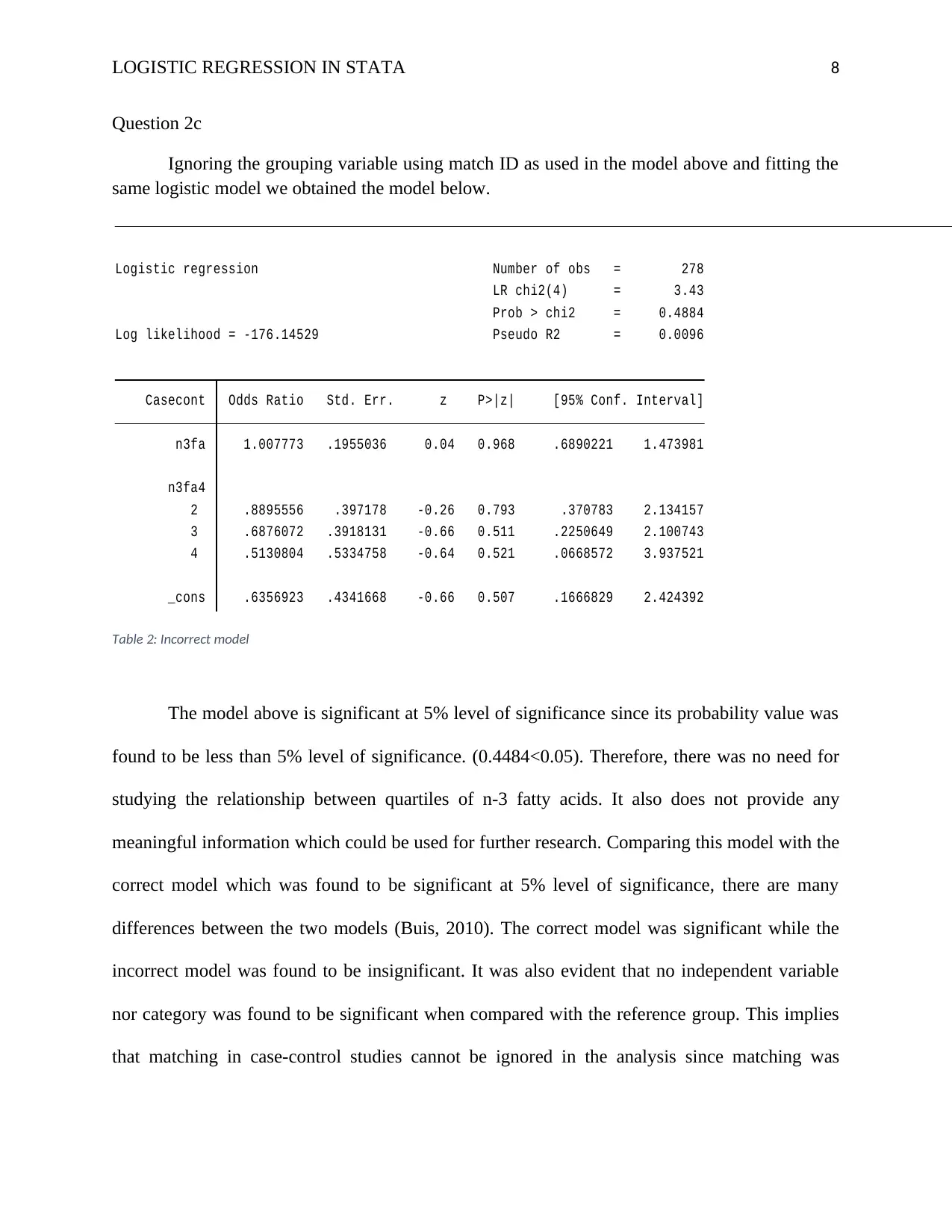
Question 2c
Ignoring the grouping variable using match ID as used in the model above and fitting the
same logistic model we obtained the model below.
_cons .6356923 .4341668 -0.66 0.507 .1666829 2.424392
4 .5130804 .5334758 -0.64 0.521 .0668572 3.937521
3 .6876072 .3918131 -0.66 0.511 .2250649 2.100743
2 .8895556 .397178 -0.26 0.793 .370783 2.134157
n3fa4
n3fa 1.007773 .1955036 0.04 0.968 .6890221 1.473981
Casecont Odds Ratio Std. Err. z P>|z| [95% Conf. Interval]
Log likelihood = -176.14529 Pseudo R2 = 0.0096
Prob > chi2 = 0.4884
LR chi2(4) = 3.43
Logistic regression Number of obs = 278
Table 2: Incorrect model
The model above is significant at 5% level of significance since its probability value was
found to be less than 5% level of significance. (0.4484<0.05). Therefore, there was no need for
studying the relationship between quartiles of n-3 fatty acids. It also does not provide any
meaningful information which could be used for further research. Comparing this model with the
correct model which was found to be significant at 5% level of significance, there are many
differences between the two models (Buis, 2010). The correct model was significant while the
incorrect model was found to be insignificant. It was also evident that no independent variable
nor category was found to be significant when compared with the reference group. This implies
that matching in case-control studies cannot be ignored in the analysis since matching was
LOGISTIC REGRESSION IN STATA 9
accomplished in the study design. Therefore, we can conclude that there was a need to control
for the confounding by the matching variables in the analysis (Williams, 2016).
accomplished in the study design. Therefore, we can conclude that there was a need to control
for the confounding by the matching variables in the analysis (Williams, 2016).
⊘ This is a preview!⊘
Do you want full access?
Subscribe today to unlock all pages.
Trusted by 1+ million students worldwide
LOGISTIC REGRESSION IN STATA
10
References
Buis, M. L. (2010). Stata tip 87: Interpretation of interactions in nonlinear models. The Stata
Journal, 10(2), 305-308
Duchesne, T., Fortin, D., & Courbin, N. (2010). Mixed conditional logistic regression for habitat
selection studies. Journal of Animal Ecology, 79(3), 548-555.
Gerds, T. A., Scheike, T. H., & Andersen, P. K. (2012). Absolute risk regression for competing
risks: interpretation, link functions, and prediction. Statistics in medicine, 31(29), 3921-
3930
Liu, D., Li, T., & Liang, D. (2014). Incorporating logistic regression to decision-theoretic rough
sets for classifications. International Journal of Approximate Reasoning, 55(1), 197-210.
Williams, R. (2016). Understanding and interpreting generalized ordered logit models. The
Journal of Mathematical Sociology, 40(1), 7-20.
1 out of 10

Your All-in-One AI-Powered Toolkit for Academic Success.
+13062052269
info@desklib.com
Available 24*7 on WhatsApp / Email
![[object Object]](/_next/static/media/star-bottom.7253800d.svg)
Unlock your academic potential
Copyright © 2020–2026 A2Z Services. All Rights Reserved. Developed and managed by ZUCOL.