MME 4450/9521 Control Systems: Optimal Control with State Feedback
VerifiedAdded on 2023/06/15
|22
|2361
|337
Homework Assignment
AI Summary
This assignment solution covers several aspects of control systems, including determining the optimal gain vector using state feedback, finding the parameter 'r' for critical damping, calculating closed-loop system poles, and verifying results using MATLAB's 'lqr' command. It also involves determining the Kalman filter gain L and estimator system poles with specified weighting matrices. Furthermore, the assignment includes a double pendulum system analysis, involving state feedback and LQR control, alongside MATLAB program implementations for each section, with detailed explanations and results. The document concludes with an analysis of white noise and Kalman filter applications, including program implementations and comparative error estimations. Desklib provides this solution along with numerous other resources to aid students in their studies.

Dell
[COMPANY NAME] [Company address]
CONTROL SYSTEM
[COMPANY NAME] [Company address]
CONTROL SYSTEM
Paraphrase This Document
Need a fresh take? Get an instant paraphrase of this document with our AI Paraphraser

Table of Contents
Question-1.................................................................................................................................1
Question -2................................................................................................................................6
Question-3...............................................................................................................................13
References...............................................................................................................................20
Question-1
Given data:
The performance index J is given by
Where r > 0 scalar parameter
(a) Optimal gain vector K
The state feedback control law is given by u = -kx
To find the value of C (sI – A)-1 B
(SI –A)-1 = adj(SI-A)det(SI-A)
C (sI – A)-1 B = [1 0][s -1 0 s+1 ] -1 [0 1 ]
= [1 0] 1s(s+1) [s+1 1 0 s ][0 1 ]
= [1 0] 1/s2+s [1 s ]
= 1/s2+s [1+0]
C (sI – A)-1 B = 1/s2+s
The above equation is representing the value of  = [1 0 1 0 ] , B =[1 0 ] , Ĉ =[1 0]
A = [0 1 0 -1 ], B = [0 1 ]
Mcx = [B, AB]
AB = [1 -1 ]
Mcx = [1 1 0 -1 ]
 = [1 0 1 0 ] , B =[1 0 ]
⊘ This is a preview!⊘
Do you want full access?
Subscribe today to unlock all pages.

Trusted by 1+ million students worldwide
Mcz = [B, ÂB]
Mcz = [0 1 1 1 ]
To find the similarity transform relating the two. It is given by
Mcz[Mcx]-1 = T
[Mcx]-1 = [1 1 0 -1 ] 1/-1 [-1 -1 0 1 ]
= [0 1 1 1 ][-1 -1 0 1 ]
T = [0 1 1 2 ]
To find the optimal gian vector K
K = ǨT
 = [1 0 1 0 ] , B =[1 0 ]
Â-BǨ =[1-k -k 1 0 ]
The desired pole polynomial is given by S2+2s+1
Now the above value is changed by
Where Ǩ = [3 1]
Now substitute the value for Ǩ in Â-BǨ equation
= [1-3 -1 1 0 ]
=[-2 -1 1 0 ]
Therefore the original feedback system is given by
K = ǨT
K = [3 1] [0 1 1 2 ]
Finally the optimal gain vector K = [-5 -3]
(b) K is critically dampled
Given
The closed loop system is given by
When K=-5
G(s) = c(s)/R(s)
= -5/s2+s-5
=-5/s2+2 ᶓ ωns+ωn2
The critically damped system ᶓ =1
The equation is given by
= -5/ s2+2 ωns+ωn2
= -5/s(s+ωn)2
The closed system with K is critically damped the given equation is
C(s) =-5/s(s+ωn)2
Paraphrase This Document
Need a fresh take? Get an instant paraphrase of this document with our AI Paraphraser
C(s) =-3/s(s+ωn)2
(c) The closed loop system poles
The given system is C(s) =-5/s(s+ωn)2
=A/s +B/(s+ωn)2 +C/(s+ ωn)
The pole values are determined by the above equation
= -1+4.582/2 = 1.791
P1 = 1.791
P2 = -2.791
(d) Part (a) and (c) using LQR command
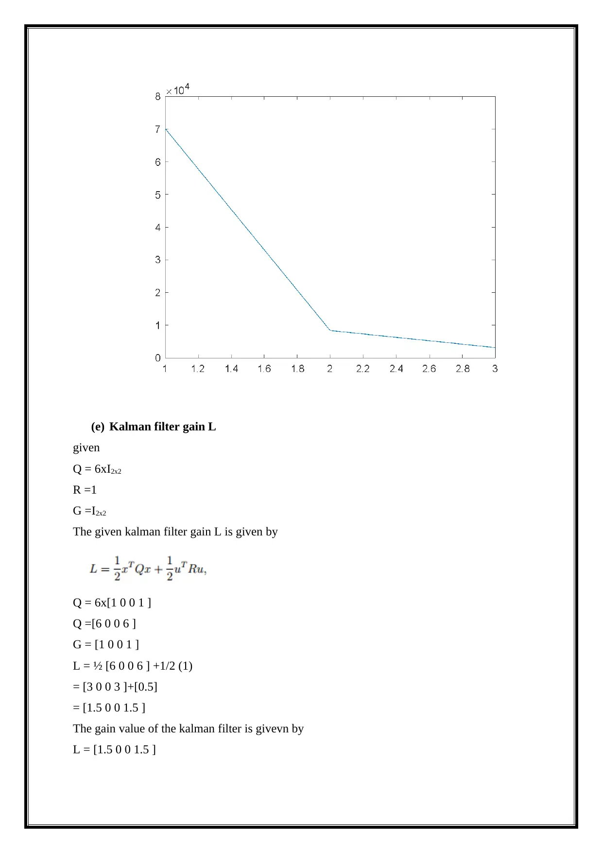
When comparing the closed loop system the below figure show in the matlab window.
This plot indicates the closed loop system poles using the LQR command
-1 -0.8 -0.6 -0.4 -0.2 0 0.2 0.4 0.6 0.8 1
n (samples)
-0.7
-0.6
-0.5
-0.4
-0.3
-0.2
-0.1
0
Amplitude
Step Response
(e) Kalman filter gain L
given
Q = 6xI2x2
R =1
G =I2x2
The given kalman filter gain L is given by
Q = 6x[1 0 0 1 ]
Q =[6 0 0 6 ]
G = [1 0 0 1 ]
L = ½ [6 0 0 6 ] +1/2 (1)
= [3 0 0 3 ]+[0.5]
= [1.5 0 0 1.5 ]
The gain value of the kalman filter is givevn by
L = [1.5 0 0 1.5 ]
given
Q = 6xI2x2
R =1
G =I2x2
The given kalman filter gain L is given by
Q = 6x[1 0 0 1 ]
Q =[6 0 0 6 ]
G = [1 0 0 1 ]
L = ½ [6 0 0 6 ] +1/2 (1)
= [3 0 0 3 ]+[0.5]
= [1.5 0 0 1.5 ]
The gain value of the kalman filter is givevn by
L = [1.5 0 0 1.5 ]
⊘ This is a preview!⊘
Do you want full access?
Subscribe today to unlock all pages.

Trusted by 1+ million students worldwide
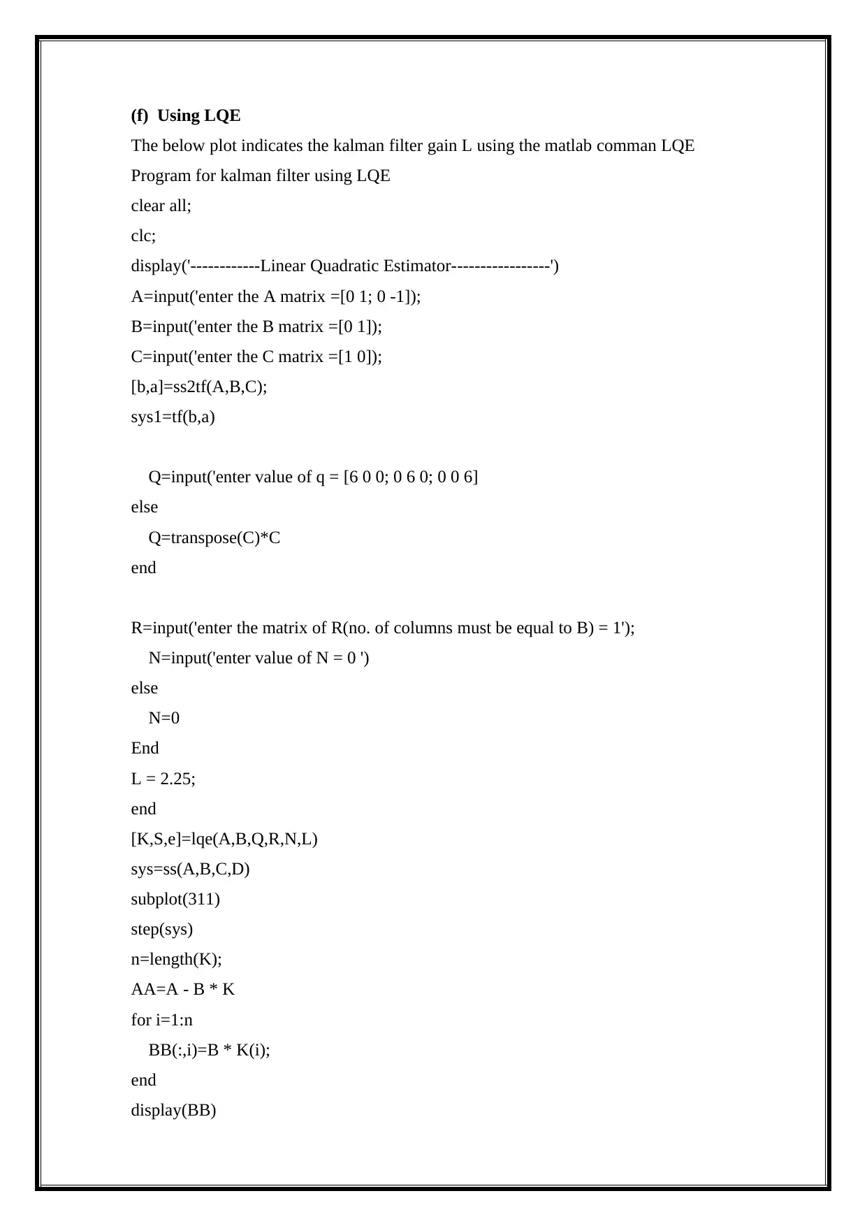
(f) Using LQE
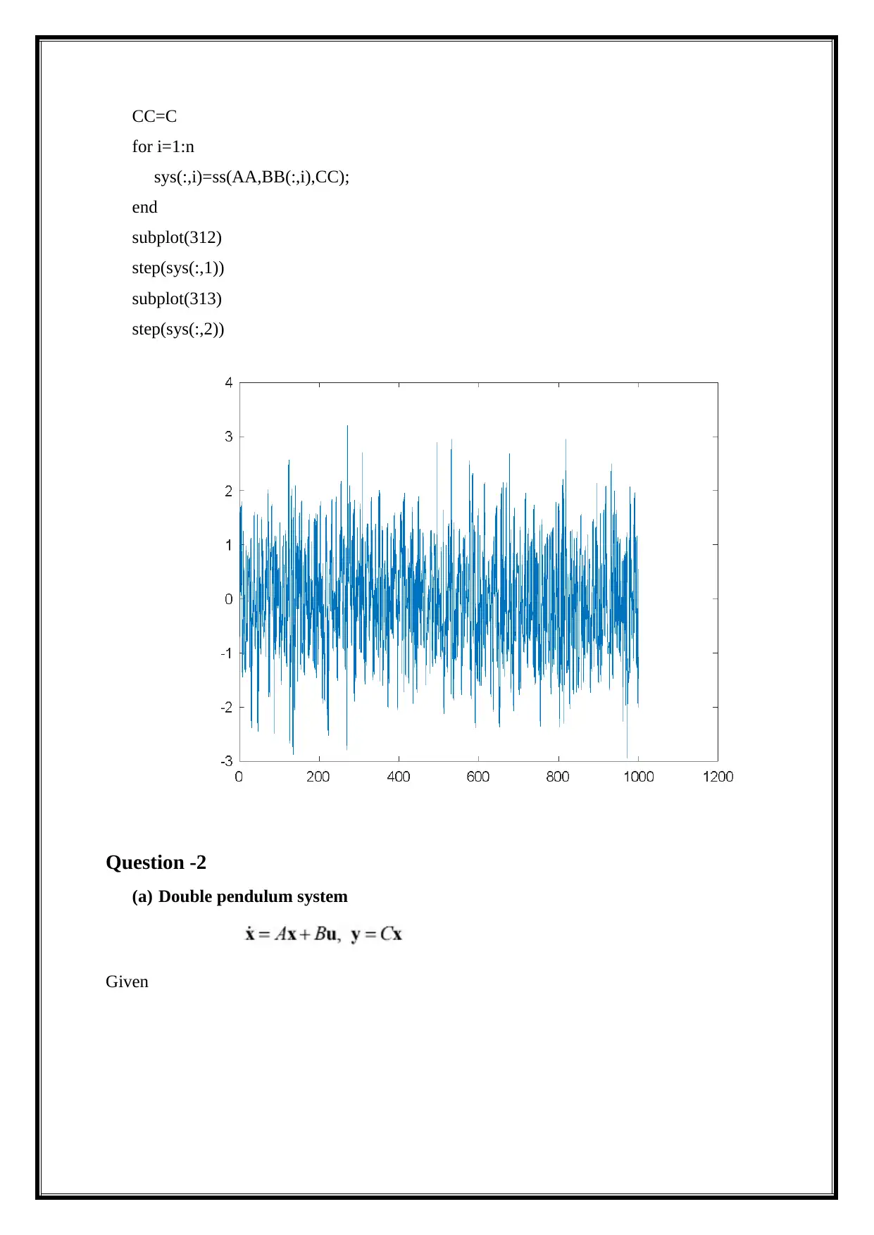
The below plot indicates the kalman filter gain L using the matlab comman LQE
Program for kalman filter using LQE
clear all;
clc;
display('------------Linear Quadratic Estimator-----------------')
A=input('enter the A matrix =[0 1; 0 -1]);
B=input('enter the B matrix =[0 1]);
C=input('enter the C matrix =[1 0]);
[b,a]=ss2tf(A,B,C);
sys1=tf(b,a)
Q=input('enter value of q = [6 0 0; 0 6 0; 0 0 6]
else
Q=transpose(C)*C
end
R=input('enter the matrix of R(no. of columns must be equal to B) = 1');
N=input('enter value of N = 0 ')
else
N=0
End
L = 2.25;
end
[K,S,e]=lqe(A,B,Q,R,N,L)
sys=ss(A,B,C,D)
subplot(311)
step(sys)
n=length(K);
AA=A - B * K
for i=1:n
BB(:,i)=B * K(i);
end
display(BB)
Paraphrase This Document
Need a fresh take? Get an instant paraphrase of this document with our AI Paraphraser
CC=C
for i=1:n
sys(:,i)=ss(AA,BB(:,i),CC);
end
subplot(312)
step(sys(:,1))
subplot(313)
step(sys(:,2))
Question -2
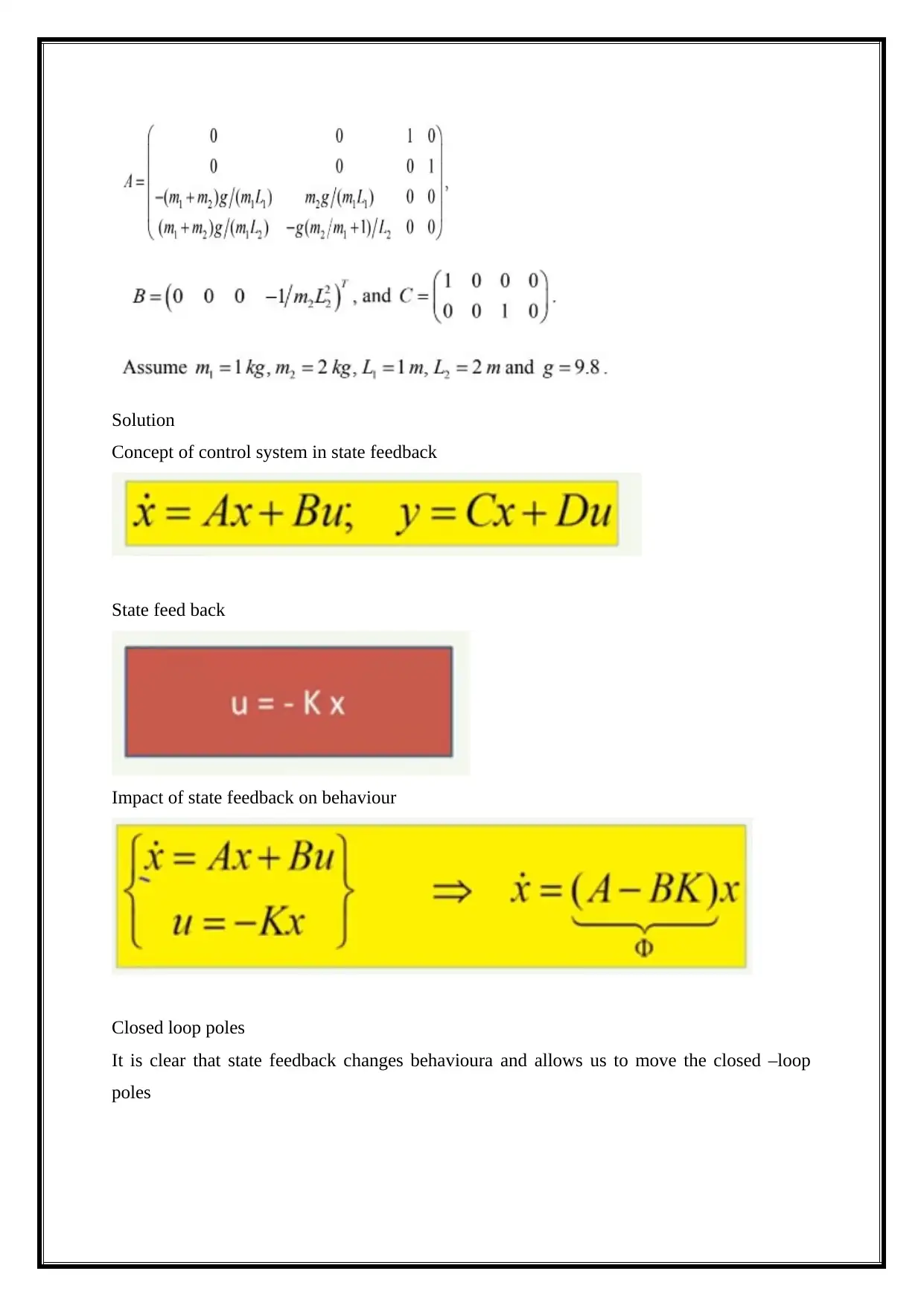
(a) Double pendulum system
Given
for i=1:n
sys(:,i)=ss(AA,BB(:,i),CC);
end
subplot(312)
step(sys(:,1))
subplot(313)
step(sys(:,2))
Question -2
(a) Double pendulum system
Given
Solution
Concept of control system in state feedback
State feed back
Impact of state feedback on behaviour
Closed loop poles
It is clear that state feedback changes behavioura and allows us to move the closed –loop
poles
Concept of control system in state feedback
State feed back
Impact of state feedback on behaviour
Closed loop poles
It is clear that state feedback changes behavioura and allows us to move the closed –loop
poles
⊘ This is a preview!⊘
Do you want full access?
Subscribe today to unlock all pages.

Trusted by 1+ million students worldwide
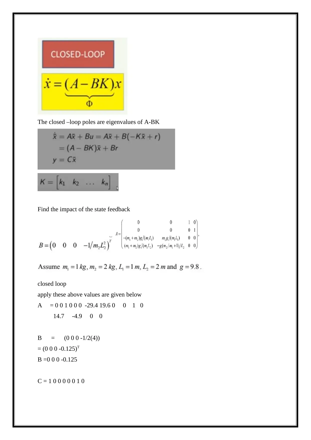
The closed –loop poles are eigenvalues of A-BK
Find the impact of the state feedback
closed loop
apply these above values are given below
A = 0 0 1 0 0 0 -29.4 19.6 0 0 1 0
14.7 -4.9 0 0
B = (0 0 0 -1/2(4))
= (0 0 0 -0.125)T
B =0 0 0 -0.125
C = 1 0 0 0 0 0 1 0
Find the impact of the state feedback
closed loop
apply these above values are given below
A = 0 0 1 0 0 0 -29.4 19.6 0 0 1 0
14.7 -4.9 0 0
B = (0 0 0 -1/2(4))
= (0 0 0 -0.125)T
B =0 0 0 -0.125
C = 1 0 0 0 0 0 1 0
Paraphrase This Document
Need a fresh take? Get an instant paraphrase of this document with our AI Paraphraser
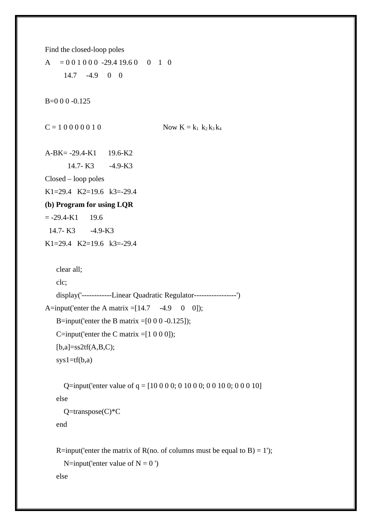
Find the closed-loop poles
A = 0 0 1 0 0 0 -29.4 19.6 0 0 1 0
14.7 -4.9 0 0
B=0 0 0 -0.125
C = 1 0 0 0 0 0 1 0 Now K = k1 k2 k3 k4
A-BK= -29.4-K1 19.6-K2
14.7- K3 -4.9-K3
Closed – loop poles
K1=29.4 K2=19.6 k3=-29.4
(b) Program for using LQR
= -29.4-K1 19.6
14.7- K3 -4.9-K3
K1=29.4 K2=19.6 k3=-29.4
clear all;
clc;
display('------------Linear Quadratic Regulator-----------------')
A=input('enter the A matrix =[14.7 -4.9 0 0]);
B=input('enter the B matrix =[0 0 0 -0.125]);
C=input('enter the C matrix =[1 0 0 0]);
[b,a]=ss2tf(A,B,C);
sys1=tf(b,a)
Q=input('enter value of q = [10 0 0 0; 0 10 0 0; 0 0 10 0; 0 0 0 10]
else
Q=transpose(C)*C
end
R=input('enter the matrix of R(no. of columns must be equal to B) = 1');
N=input('enter value of N = 0 ')
else
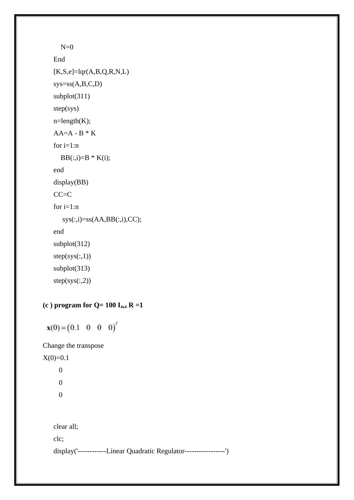
N=0
End
[K,S,e]=lqr(A,B,Q,R,N,L)
sys=ss(A,B,C,D)
subplot(311)
step(sys)
n=length(K);
AA=A - B * K
for i=1:n
BB(:,i)=B * K(i);
end
display(BB)
CC=C
for i=1:n
sys(:,i)=ss(AA,BB(:,i),CC);
end
subplot(312)
step(sys(:,1))
subplot(313)
step(sys(:,2))
(c ) program for Q= 100 I4x4 R =1
Change the transpose
X(0)=0.1
0
0
0
clear all;
clc;
display('------------Linear Quadratic Regulator-----------------')
⊘ This is a preview!⊘
Do you want full access?
Subscribe today to unlock all pages.

Trusted by 1+ million students worldwide
1 out of 22
Related Documents
Your All-in-One AI-Powered Toolkit for Academic Success.
+13062052269
info@desklib.com
Available 24*7 on WhatsApp / Email
![[object Object]](/_next/static/media/star-bottom.7253800d.svg)
Unlock your academic potential
Copyright © 2020–2026 A2Z Services. All Rights Reserved. Developed and managed by ZUCOL.


