Analysis of Station Usage Data: Eccleston Park (2009-2018) Report

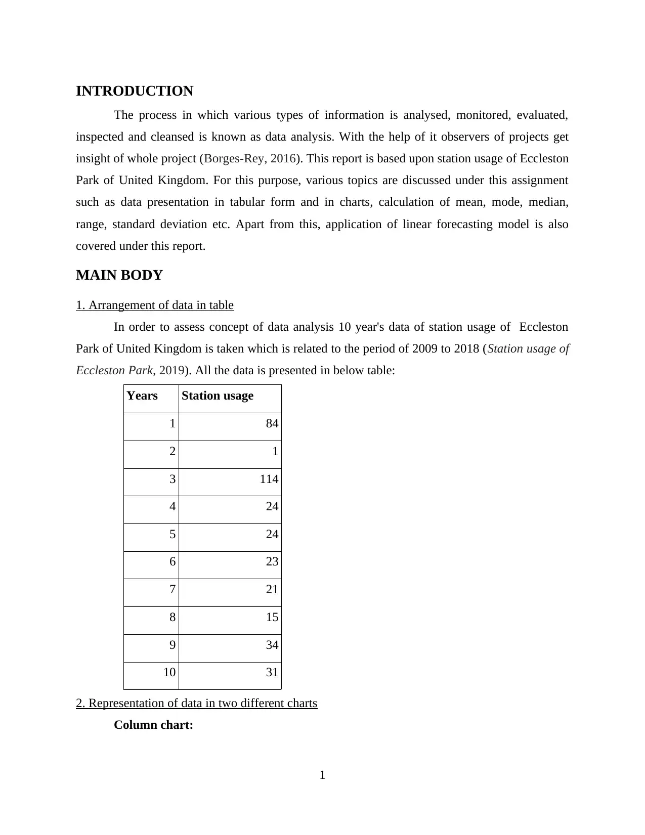
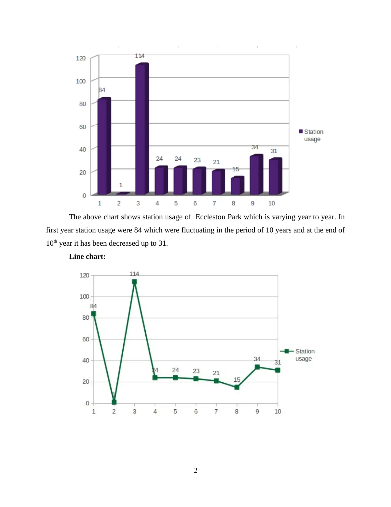
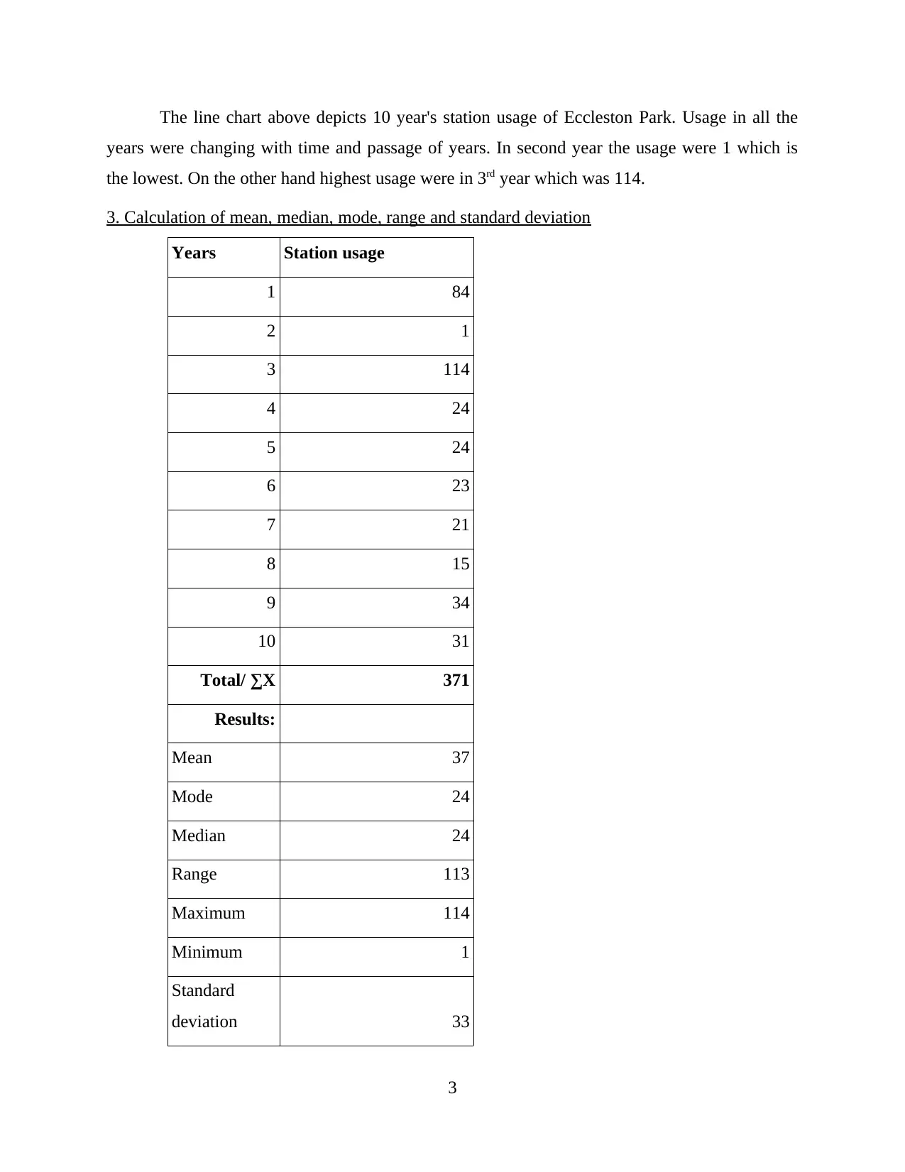
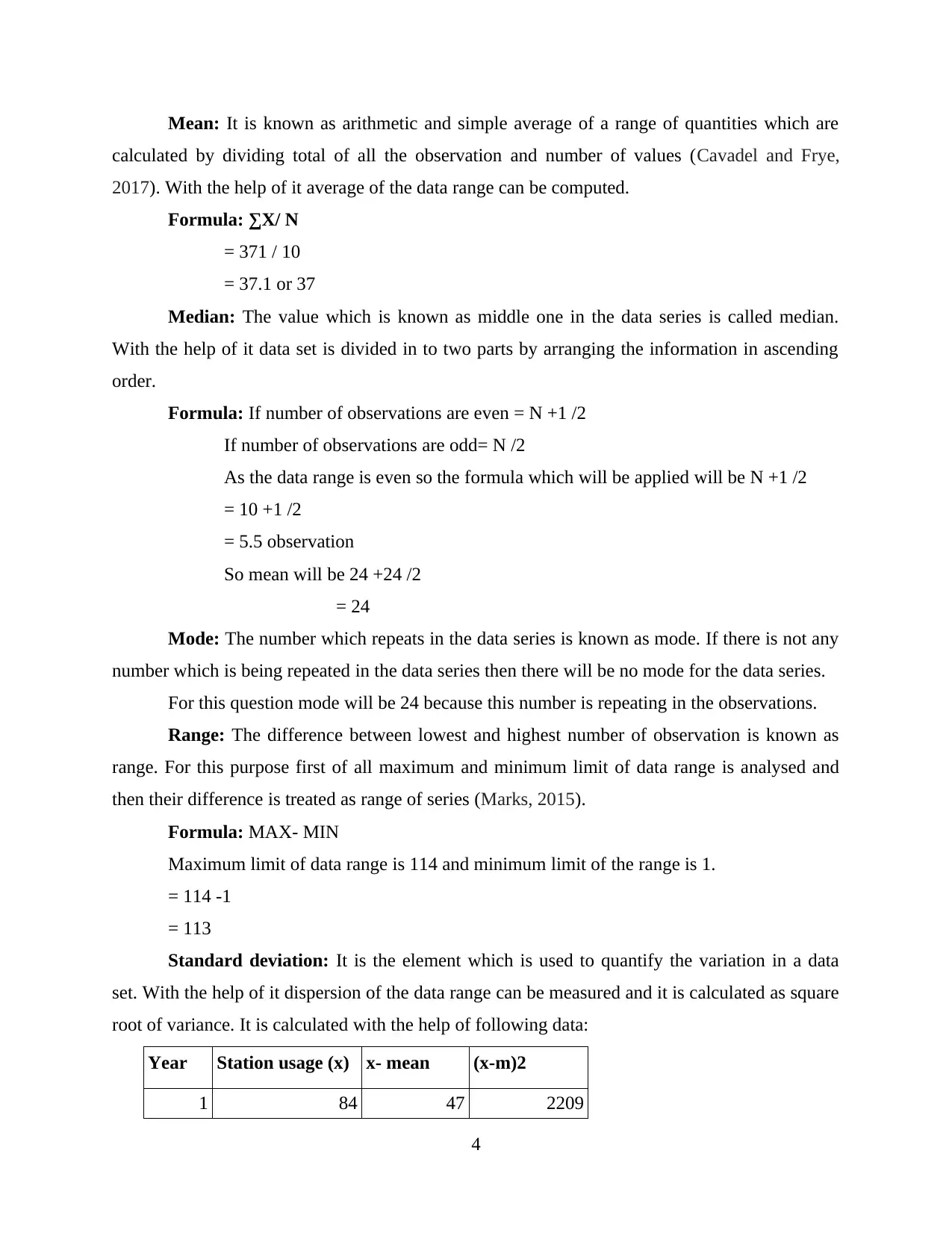
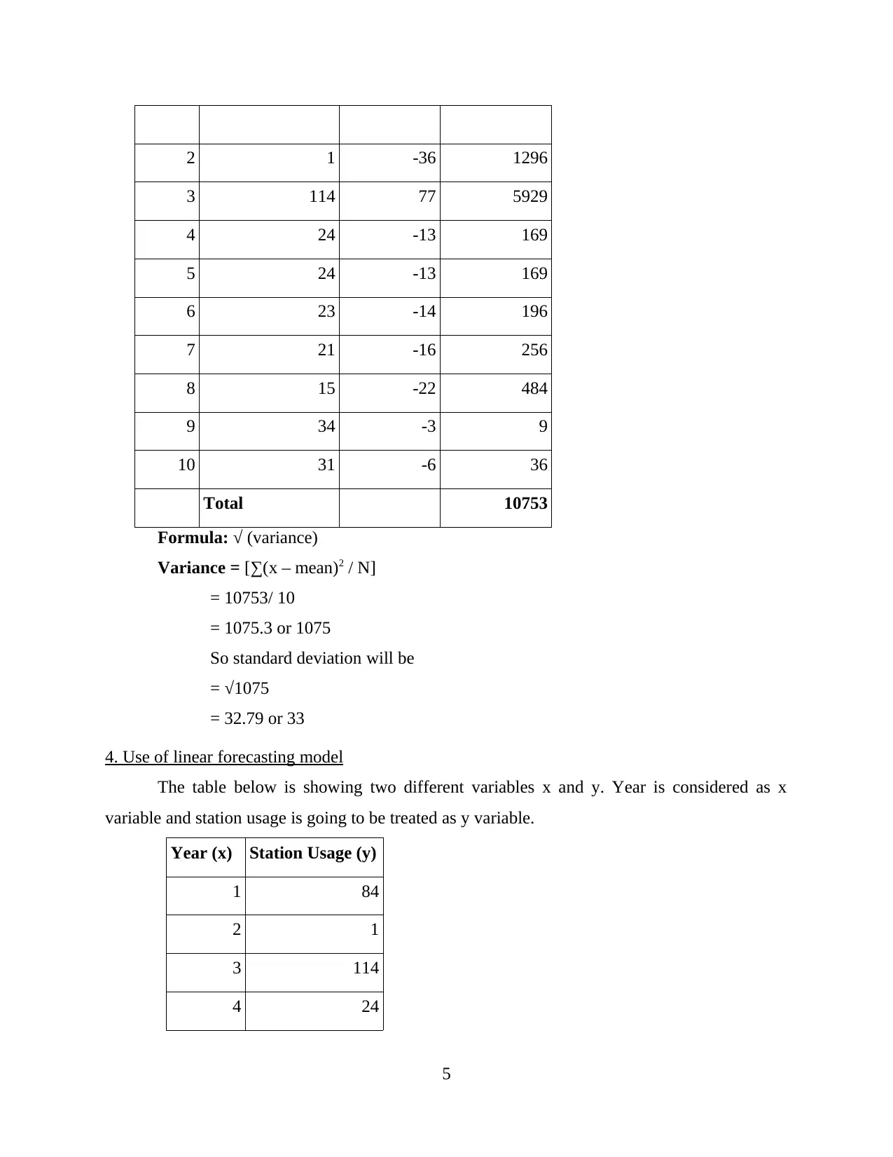
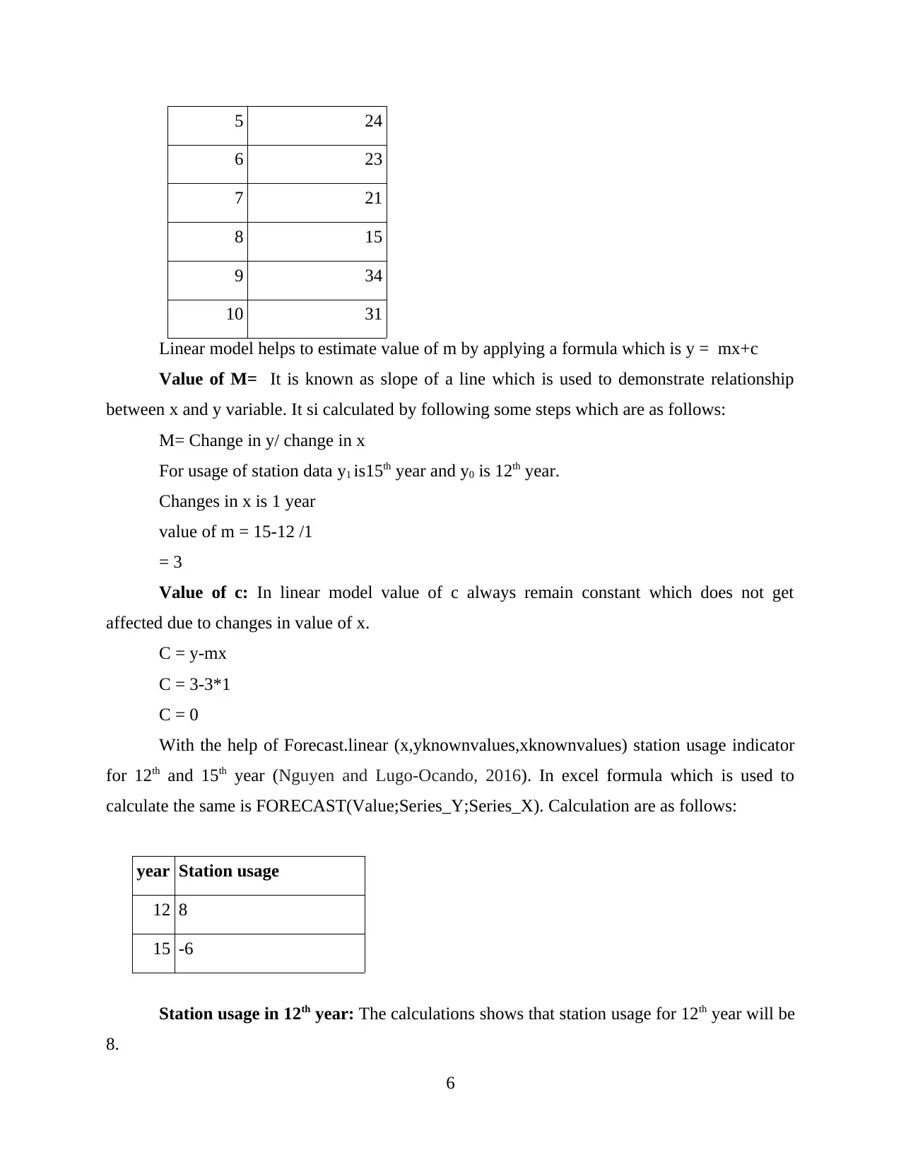
This report provides a comprehensive data analysis of Eccleston Park station usage from 2009 to 2018. It begins with an introduction to data analysis, followed by a presentation of the data in tabular form. The report includes the use of column and line charts to visually represent the data. Furthermore, it calculates and explains key statistical measures such as mean, median, mode, range, and standard deviation. A significant part of the report focuses on the application of a linear forecasting model to predict future station usage. The report concludes with a summary of the findings and a list of cited references. This report is designed to demonstrate the application of various data analysis techniques to real-world data, providing valuable insights into station usage trends.

Numeracy and Data
Analysis

Table of Contents
INTRODUCTION...........................................................................................................................1
MAIN BODY...................................................................................................................................1
1. Arrangement of data in table....................................................................................................1
2. Representation of data in two different charts.........................................................................1
3. Calculation of mean, median, mode, range and standard deviation........................................3
4. Use of linear forecasting model...............................................................................................5
CONCLUSION................................................................................................................................6
REFERENCES................................................................................................................................7

INTRODUCTION
The process in which various types of information is analysed, monitored, evaluated,
inspected and cleansed is known as data analysis. With the help of it observers of projects get
insight of whole project (Borges-Rey, 2016). This report is based upon station usage of Eccleston
Park of United Kingdom. For this purpose, various topics are discussed under this assignment
such as data presentation in tabular form and in charts, calculation of mean, mode, median,
range, standard deviation etc. Apart from this, application of linear forecasting model is also
covered under this report.
MAIN BODY
1. Arrangement of data in table
In order to assess concept of data analysis 10 year's data of station usage of Eccleston
Park of United Kingdom is taken which is related to the period of 2009 to 2018 (Station usage of
Eccleston Park, 2019). All the data is presented in below table:
Years Station usage
1 84
2 1
3 114
4 24
5 24
6 23
7 21
8 15
9 34
10 31
2. Representation of data in two different charts
Column chart:
1

The above chart shows station usage of Eccleston Park which is varying year to year. In
first year station usage were 84 which were fluctuating in the period of 10 years and at the end of
10th year it has been decreased up to 31.
Line chart:
2

The line chart above depicts 10 year's station usage of Eccleston Park. Usage in all the
years were changing with time and passage of years. In second year the usage were 1 which is
the lowest. On the other hand highest usage were in 3rd year which was 114.
3. Calculation of mean, median, mode, range and standard deviation
Years Station usage
1 84
2 1
3 114
4 24
5 24
6 23
7 21
8 15
9 34
10 31
Total/ ∑X 371
Results:
Mean 37
Mode 24
Median 24
Range 113
Maximum 114
Minimum 1
Standard
deviation 33
3

Mean: It is known as arithmetic and simple average of a range of quantities which are
calculated by dividing total of all the observation and number of values (Cavadel and Frye,
2017). With the help of it average of the data range can be computed.
Formula: ∑X/ N
= 371 / 10
= 37.1 or 37
Median: The value which is known as middle one in the data series is called median.
With the help of it data set is divided in to two parts by arranging the information in ascending
order.
Formula: If number of observations are even = N +1 /2
If number of observations are odd= N /2
As the data range is even so the formula which will be applied will be N +1 /2
= 10 +1 /2
= 5.5 observation
So mean will be 24 +24 /2
= 24
Mode: The number which repeats in the data series is known as mode. If there is not any
number which is being repeated in the data series then there will be no mode for the data series.
For this question mode will be 24 because this number is repeating in the observations.
Range: The difference between lowest and highest number of observation is known as
range. For this purpose first of all maximum and minimum limit of data range is analysed and
then their difference is treated as range of series (Marks, 2015).
Formula: MAX- MIN
Maximum limit of data range is 114 and minimum limit of the range is 1.
= 114 -1
= 113
Standard deviation: It is the element which is used to quantify the variation in a data
set. With the help of it dispersion of the data range can be measured and it is calculated as square
root of variance. It is calculated with the help of following data:
Year Station usage (x) x- mean (x-m)2
1 84 47 2209
4

2 1 -36 1296
3 114 77 5929
4 24 -13 169
5 24 -13 169
6 23 -14 196
7 21 -16 256
8 15 -22 484
9 34 -3 9
10 31 -6 36
Total 10753
Formula: √ (variance)
Variance = [∑(x – mean)2 / N]
= 10753/ 10
= 1075.3 or 1075
So standard deviation will be
= √1075
= 32.79 or 33
4. Use of linear forecasting model
The table below is showing two different variables x and y. Year is considered as x
variable and station usage is going to be treated as y variable.
Year (x) Station Usage (y)
1 84
2 1
3 114
4 24
5

5 24
6 23
7 21
8 15
9 34
10 31
Linear model helps to estimate value of m by applying a formula which is y = mx+c
Value of M= It is known as slope of a line which is used to demonstrate relationship
between x and y variable. It si calculated by following some steps which are as follows:
M= Change in y/ change in x
For usage of station data y1 is15th year and y0 is 12th year.
Changes in x is 1 year
value of m = 15-12 /1
= 3
Value of c: In linear model value of c always remain constant which does not get
affected due to changes in value of x.
C = y-mx
C = 3-3*1
C = 0
With the help of Forecast.linear (x,yknownvalues,xknownvalues) station usage indicator
for 12th and 15th year (Nguyen and Lugo-Ocando, 2016). In excel formula which is used to
calculate the same is FORECAST(Value;Series_Y;Series_X). Calculation are as follows:
year Station usage
12 8
15 -6
Station usage in 12th year: The calculations shows that station usage for 12th year will be
8.
6

Station usage in 15th year: For 15th year station usage will be -6.
CONCLUSION
From the above project report it has been concluded that data analysis helps to get insight
in to the information which is being collected by researcher. With the help of different tools such
as mean, mode, median, range, standard deviation and linear model data analysis can be
conducted in appropriate manner.
7