Statistical Analysis Homework: Hypothesis Testing, Regression Analysis

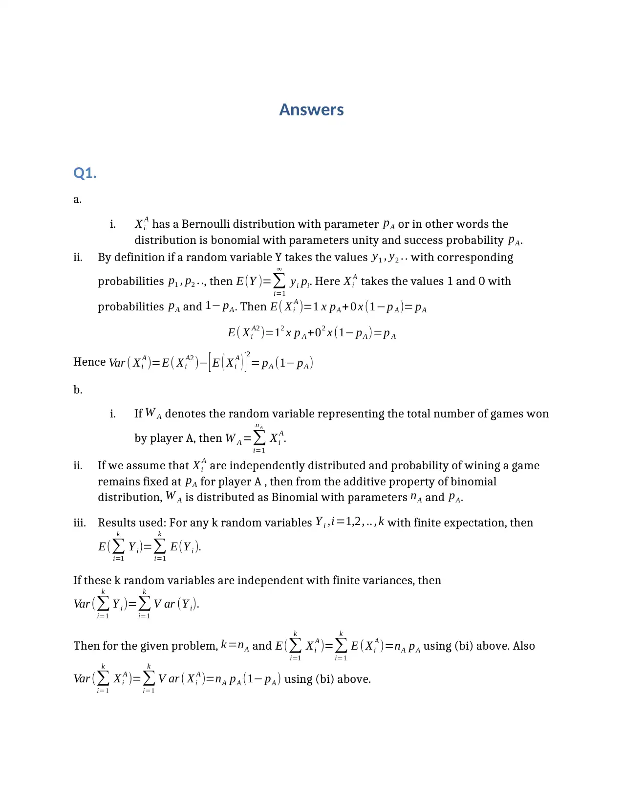
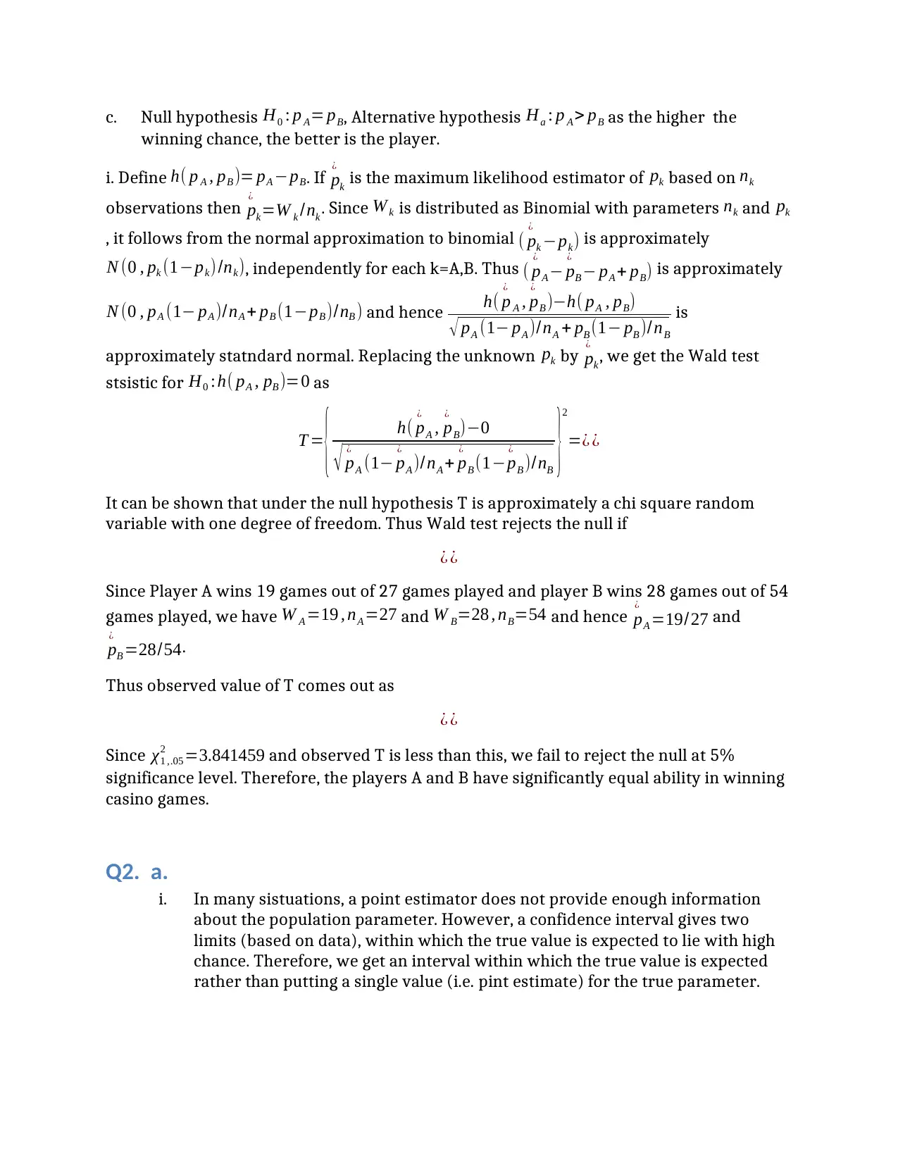
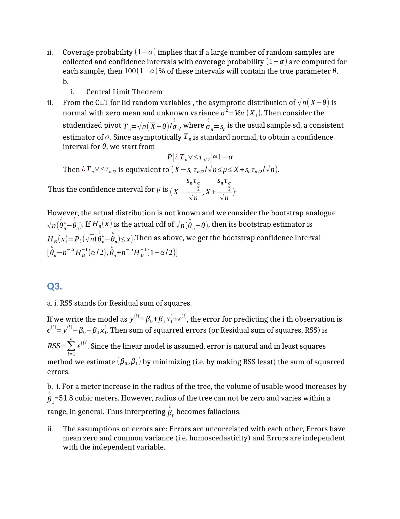
This document provides a detailed solution to a statistics homework assignment. The solution begins with an analysis of probability distributions, including Bernoulli and binomial distributions, and applies these concepts to a hypothesis testing problem involving the comparison of player abilities in a casino game. It then delves into the concept of confidence intervals, explaining their importance in providing a range of plausible values for a population parameter, and discusses the Central Limit Theorem and bootstrap methods for constructing confidence intervals. The assignment also covers regression analysis, explaining the concept of Residual Sum of Squares (RSS) and interpreting the coefficients of a linear regression model. It includes an analysis of the assumptions of linear regression and identifies potential outliers, providing suggestions for improving the model. The document aims to provide students with a comprehensive understanding of statistical concepts and their applications.

Answers
Q1.
a.
i. Xi
A has a Bernoulli distribution with parameter pA or in other words the
distribution is bonomial with parameters unity and success probability pA.
ii. By definition if a random variable Y takes the values y1 , y2 . . with corresponding
probabilities p1 , p2 . ., then E(Y )=∑
i=1
∞
yi pi. Here Xi
A takes the values 1 and 0 with
probabilities pA and 1− pA . Then E( Xi
A )=1 x pA + 0 x (1−p A )= pA
E( Xi
A2 )=12 x p A +02 x (1− pA )=p A
Hence Var ( Xi
A )=E( Xi
A2 )− [ E ( Xi
A ) ]
2
= pA (1− pA )
b.
i. If W A denotes the random variable representing the total number of games won
by player A, then W A =∑
i=1
n A
Xi
A.
ii. If we assume that Xi
A are independently distributed and probability of wining a game
remains fixed at pA for player A , then from the additive property of binomial
distribution, W A is distributed as Binomial with parameters nA and pA.
iii. Results used: For any k random variables Y i ,i=1,2, .. , k with finite expectation, then
E(∑
i=1
k
Y i)=∑
i=1
k
E(Y i ).
If these k random variables are independent with finite variances, then
Var (∑
i=1
k
Y i )=∑
i=1
k
V ar (Y i).
Then for the given problem, k =nA and E(∑
i=1
k
Xi
A )=∑
i=1
k
E ( Xi
A )=nA pA using (bi) above. Also
Var (∑
i=1
k
Xi
A )=∑
i=1
k
V ar ( Xi
A )=nA pA (1− pA ) using (bi) above.

c. Null hypothesis H0 : p A= pB, Alternative hypothesis Ha : p A > pB as the higher the
winning chance, the better is the player.
i. Define h( p A , pB )= pA −pB. If p
¿
k is the maximum likelihood estimator of pk based on nk
observations then p
¿
k=W k /nk . Since W k is distributed as Binomial with parameters nk and pk
, it follows from the normal approximation to binomial ( p
¿
k −pk) is approximately
N (0 , pk (1−pk) /nk), independently for each k=A,B. Thus ( p
¿
A − p
¿
B − pA + pB) is approximately
N (0 , pA (1− pA )/nA + pB (1−pB )/nB ) and hence h( p
¿
A , p
¿
B )−h( pA , pB)
√ pA (1− pA )/nA + pB (1− pB )/nB
is
approximately statndard normal. Replacing the unknown pk by p
¿
k, we get the Wald test
stsistic for H0 :h( pA , pB )=0 as
T = { h( p
¿
A , p
¿
B)−0
√ p
¿
A (1− p
¿
A )/nA + p
¿
B (1−p
¿
B )/nB
}2
=¿ ¿
It can be shown that under the null hypothesis T is approximately a chi square random
variable with one degree of freedom. Thus Wald test rejects the null if
¿ ¿
Since Player A wins 19 games out of 27 games played and player B wins 28 games out of 54
games played, we have W A =19 , nA =27 and W B=28 , nB=54 and hence p
¿
A =19/27 and
p
¿
B =28/54.
Thus observed value of T comes out as
¿ ¿
Since χ1 ,.05
2 =3.841459 and observed T is less than this, we fail to reject the null at 5%
significance level. Therefore, the players A and B have significantly equal ability in winning
casino games.
Q2. a.
i. In many sistuations, a point estimator does not provide enough information
about the population parameter. However, a confidence interval gives two
limits (based on data), within which the true value is expected to lie with high
chance. Therefore, we get an interval within which the true value is expected
rather than putting a single value (i.e. pint estimate) for the true parameter.

ii. Coverage probability (1−α ) implies that if a large number of random samples are
collected and confidence intervals with coverage probability (1−α ) are computed for
each sample, then 100(1−α) % of these intervals will contain the true parameter θ.
b.
i. Central Limit Theorem
ii. From the CLT for iid random variables , the asymptotic distribution of √ n( X−θ) is
normal with zero mean and unknown variance σ 2=Var ( X1 ). Then consider the
studentized pivot T n= √ n( X−θ)/σ
¿
n, where σ
¿
n=sn is the usual sample sd, a consistent
estimator of σ . Since asymptotically T n is standard normal, to obtain a confidence
interval for θ, we start from
P {¿ T n∨≤ τα/ 2 } ≈1−α
Then ¿ T n∨≤ τα /2 is equivalent to (X −sn τα /2 / √ n ≤ μ ≤ X + sn τα /2 / √ n).
Thus the confidence interval for μ is ( X −
sn τ α
2
√ n , X +
sn τ α
2
√ n ).
However, the actual distribution is not known and we consider the bootstrap analogue
√n(θ
¿
n
¿−θ
¿
n ). If Hn ( x ) is the actual cdf of √n(θ
¿
n−θ), then its bootstrap estimator is
HB ( x)=P¿ ( √ n(θ
¿
n
¿−θ
¿
n )≤ x).Then as above, we get the bootstrap confidence interval
[θ
¿
n−n−.5 HB
−1 (α /2), θ
¿
n +n−.5 H B
−1 (1−α /2)]
Q3.
a. i. RSS stands for Residual sum of squares.
If we write the model as y(i )=β0 + β1 x1
i + ϵ(i), the error for predicting the i th observation is
ϵ(i )= y(i )−β0−β1 x1
i . Then sum of squarred errors (or Residual sum of squares, RSS) is
RSS=∑
i=1
n
ϵ(i)2
. Since the linear model is assumed, error is natural and in least squares
method we estimate ( β0 , β1 ) by minimizing (i.e. by making RSS least) the sum of squarred
errors.
b. i. For a meter increase in the radius of the tree, the volume of usable wood increases by
β
¿
1=51.8 cubic meters. However, radius of the tree can not be zero and varies within a
range, in general. Thus interpreting β
¿
0 becomes fallacious.
ii. The assumptions on errors are: Errors are uncorrelated with each other, Errors have
mean zero and common variance (i.e. homoscedasticity) and Errors are independent
with the independent variable.

From the second plot, we observe that residuals vary about zero symmetrically and hence
linear relationship is reasonable, which is also supported by the first plot. The residuals
almost form a “horizontal band” around the 0 line. Thus the spread of the residuals remains
fixed and this suggests that the variances of the error terms are equal. Thus constant
variance of error seems to be satisfied together with zero mean assumption. However, the
last residual seems odd to the basic pattern of residuals. The first figure also show that the
corresponding observation is distant from the fitted line. This suggests that the observation
is an outlier.
c. i. However, for a potentially better model, the merchant could delete the outlier and re
run the regression on the remaining observations.
ii. Since radius is not uniform, the girth weight should me measured further to include in
the model. The girth weight explains the average weight related to the measured
radius and seems useful in addition to other covariate.