Statistics for Management: Data Analysis and Report, 2024
VerifiedAdded on 2020/10/22
|15
|3039
|334
Report
AI Summary
This report presents a statistical analysis of various management aspects. It begins with an examination of earnings differences between men and women in both public and private sectors, utilizing t-tests to determine significance. The report then employs ogive charts to analyze hourly earnings distribution and compares earnings in London and Manchester. Further, it delves into inventory management, calculating economic order quantity, reorder levels, and service levels. Finally, the report includes a graphical representation of CPI, CPIH, and RPI from 2007-2017, offering insights into inflation trends, and concludes with an ogive chart analysis of cumulative staff percentages versus hourly earnings.

Statistics for
Management
Management
Paraphrase This Document
Need a fresh take? Get an instant paraphrase of this document with our AI Paraphraser
Table of Contents
INTRODUCTION...........................................................................................................................1
Activity 1.........................................................................................................................................1
A) Determining the earnings of men and women in public sector.............................................1
B) Determining the earnings of men and women in private sector.............................................2
C) Earning time chart..................................................................................................................3
Gross annual earnings of male of public and private sector ......................................................3
.....................................................................................................................................................3
Gross annual earnings of female of public and private sector ...................................................3
D) Determination of annual growth rate in earnings..................................................................4
Activity 2.........................................................................................................................................5
2A................................................................................................................................................5
I) Use of ogive chart median hourly earnings along the quartile................................................5
II) Calculation of the mean and standard deviation for hourly earnings.....................................7
2B. Comparison of the earning in London and Manchester......................................................8
Activity 3.........................................................................................................................................9
A) Economic order quantity........................................................................................................9
B) Intervals for ordering T-Shirts...............................................................................................9
C) Inventory policy cost..............................................................................................................9
D) Current service level to customers.........................................................................................9
E) Re-order level to achieve the desired service level................................................................9
Activity 4.......................................................................................................................................10
a) Graphical representation of CPI, CPIH and RPI from 2007-2017.......................................10
...................................................................................................................................................11
b) presentation of the Ogive chart for cumulative % of staff versus the hourly earnings.........12
CONCLUSION..............................................................................................................................12
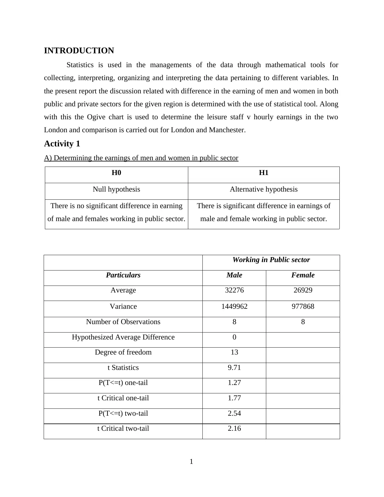
INTRODUCTION
Statistics is used in the managements of the data through mathematical tools for
collecting, interpreting, organizing and interpreting the data pertaining to different variables. In
the present report the discussion related with difference in the earning of men and women in both
public and private sectors for the given region is determined with the use of statistical tool. Along
with this the Ogive chart is used to determine the leisure staff v hourly earnings in the two
London and comparison is carried out for London and Manchester.
Activity 1
A) Determining the earnings of men and women in public sector
H0 H1
Null hypothesis Alternative hypothesis
There is no significant difference in earning
of male and females working in public sector.
There is significant difference in earnings of
male and female working in public sector.
Working in Public sector
Particulars Male Female
Average 32276 26929
Variance 1449962 977868
Number of Observations 8 8
Hypothesized Average Difference 0
Degree of freedom 13
t Statistics 9.71
P(T<=t) one-tail 1.27
t Critical one-tail 1.77
P(T<=t) two-tail 2.54
t Critical two-tail 2.16
1
⊘ This is a preview!⊘
Do you want full access?
Subscribe today to unlock all pages.
Trusted by 1+ million students worldwide
Interpretation: from the above calculating it can be interpreted that the earnings in the
public sectors for both men and females are different (Baak and et.al., 2015). The valve of p in
the above case is higher than 0.5 which accepts the null hypothesis stating the fact that there is no
significant relation in the earnings of the men and the female in the public sector with an average
earning of male as 32276 and of female as 26929.
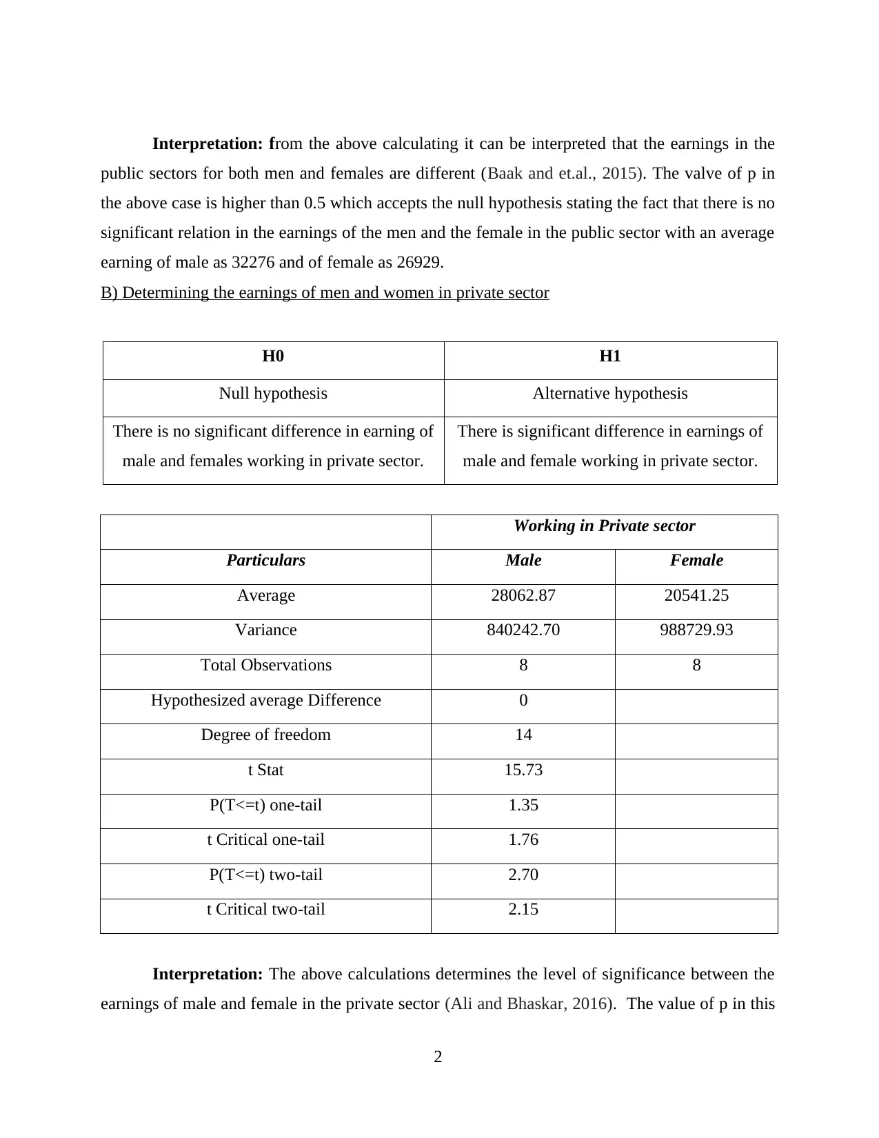
B) Determining the earnings of men and women in private sector
H0 H1
Null hypothesis Alternative hypothesis
There is no significant difference in earning of
male and females working in private sector.
There is significant difference in earnings of
male and female working in private sector.
Working in Private sector
Particulars Male Female
Average 28062.87 20541.25
Variance 840242.70 988729.93
Total Observations 8 8
Hypothesized average Difference 0
Degree of freedom 14
t Stat 15.73
P(T<=t) one-tail 1.35
t Critical one-tail 1.76
P(T<=t) two-tail 2.70
t Critical two-tail 2.15
Interpretation: The above calculations determines the level of significance between the
earnings of male and female in the private sector (Ali and Bhaskar, 2016). The value of p in this
2
public sectors for both men and females are different (Baak and et.al., 2015). The valve of p in
the above case is higher than 0.5 which accepts the null hypothesis stating the fact that there is no
significant relation in the earnings of the men and the female in the public sector with an average
earning of male as 32276 and of female as 26929.
B) Determining the earnings of men and women in private sector
H0 H1
Null hypothesis Alternative hypothesis
There is no significant difference in earning of
male and females working in private sector.
There is significant difference in earnings of
male and female working in private sector.
Working in Private sector
Particulars Male Female
Average 28062.87 20541.25
Variance 840242.70 988729.93
Total Observations 8 8
Hypothesized average Difference 0
Degree of freedom 14
t Stat 15.73
P(T<=t) one-tail 1.35
t Critical one-tail 1.76
P(T<=t) two-tail 2.70
t Critical two-tail 2.15
Interpretation: The above calculations determines the level of significance between the
earnings of male and female in the private sector (Ali and Bhaskar, 2016). The value of p in this
2
Paraphrase This Document
Need a fresh take? Get an instant paraphrase of this document with our AI Paraphraser
case also is more than 0.5 at 2.15 which leads to acceptance of the null hypothesis with stating
the facts there is significance level is absent in the earning level of both male and females in the
private sector as well.
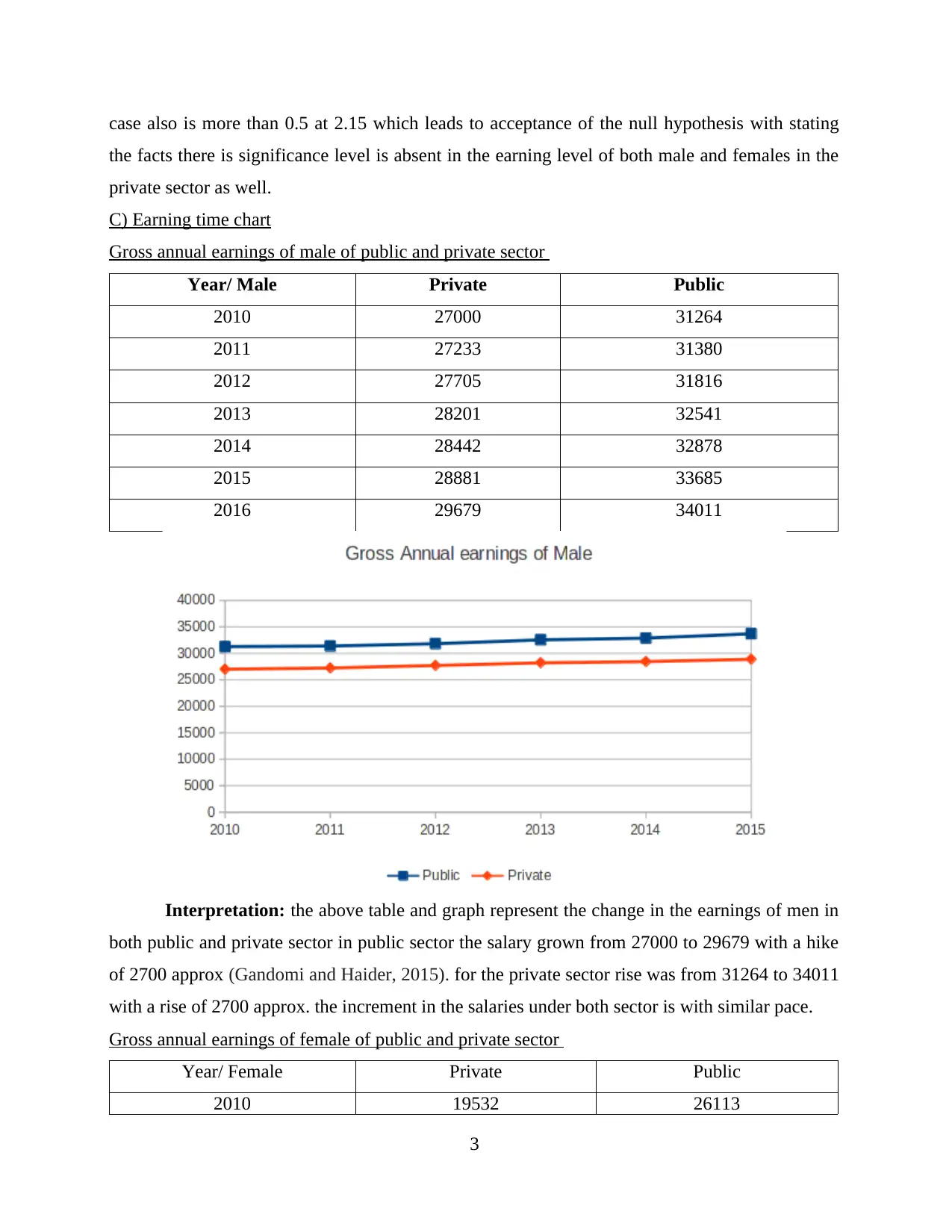
C) Earning time chart
Gross annual earnings of male of public and private sector
Year/ Male Private Public
2010 27000 31264
2011 27233 31380
2012 27705 31816
2013 28201 32541
2014 28442 32878
2015 28881 33685
2016 29679 34011
Interpretation: the above table and graph represent the change in the earnings of men in
both public and private sector in public sector the salary grown from 27000 to 29679 with a hike
of 2700 approx (Gandomi and Haider, 2015). for the private sector rise was from 31264 to 34011
with a rise of 2700 approx. the increment in the salaries under both sector is with similar pace.
Gross annual earnings of female of public and private sector
Year/ Female Private Public
2010 19532 26113
3
the facts there is significance level is absent in the earning level of both male and females in the
private sector as well.
C) Earning time chart
Gross annual earnings of male of public and private sector
Year/ Male Private Public
2010 27000 31264
2011 27233 31380
2012 27705 31816
2013 28201 32541
2014 28442 32878
2015 28881 33685
2016 29679 34011
Interpretation: the above table and graph represent the change in the earnings of men in
both public and private sector in public sector the salary grown from 27000 to 29679 with a hike
of 2700 approx (Gandomi and Haider, 2015). for the private sector rise was from 31264 to 34011
with a rise of 2700 approx. the increment in the salaries under both sector is with similar pace.
Gross annual earnings of female of public and private sector
Year/ Female Private Public
2010 19532 26113
3
2011 19565 26470
2012 20313 26636
2013 20698 27338
2014 21017 27705
2015 21403 27905
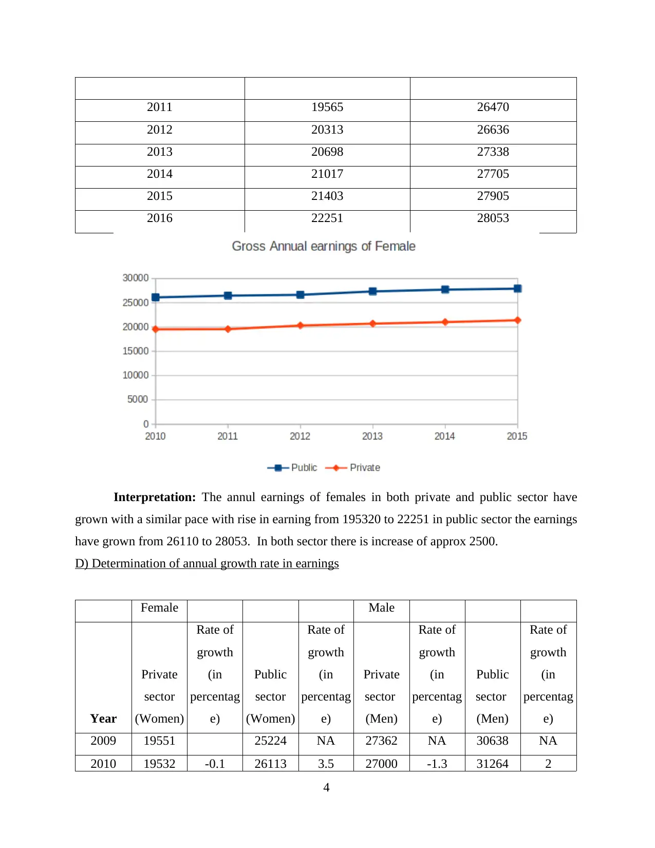
2016 22251 28053
Interpretation: The annul earnings of females in both private and public sector have
grown with a similar pace with rise in earning from 195320 to 22251 in public sector the earnings
have grown from 26110 to 28053. In both sector there is increase of approx 2500.
D) Determination of annual growth rate in earnings
Female Male
Year
Private
sector
(Women)
Rate of
growth
(in
percentag
e)
Public
sector
(Women)
Rate of
growth
(in
percentag
e)
Private
sector
(Men)
Rate of
growth
(in
percentag
e)
Public
sector
(Men)
Rate of
growth
(in
percentag
e)
2009 19551 25224 NA 27362 NA 30638 NA
2010 19532 -0.1 26113 3.5 27000 -1.3 31264 2
4
2012 20313 26636
2013 20698 27338
2014 21017 27705
2015 21403 27905
2016 22251 28053
Interpretation: The annul earnings of females in both private and public sector have
grown with a similar pace with rise in earning from 195320 to 22251 in public sector the earnings
have grown from 26110 to 28053. In both sector there is increase of approx 2500.
D) Determination of annual growth rate in earnings
Female Male
Year
Private
sector
(Women)
Rate of
growth
(in
percentag
e)
Public
sector
(Women)
Rate of
growth
(in
percentag
e)
Private
sector
(Men)
Rate of
growth
(in
percentag
e)
Public
sector
(Men)
Rate of
growth
(in
percentag
e)
2009 19551 25224 NA 27362 NA 30638 NA
2010 19532 -0.1 26113 3.5 27000 -1.3 31264 2
4
⊘ This is a preview!⊘
Do you want full access?
Subscribe today to unlock all pages.
Trusted by 1+ million students worldwide
2011 19565 0.2 26470 1.4 27233 0.9 31380 0.4
2012 20313 3.8 26636 0.6 27705 1.7 31816 1.4
2013 20698 1.9 27338 2.6 28201 1.8 32541 2.3
2014 21017 1.5 27705 1.3 28442 0.9 32878 1
2015 21403 1.8 27900 0.7 28881 1.5 33685 2.5
2016 22251 4 28053 0.5 29679 2.8 34011 1
Interpretation: this table represent the growth in the income of both male and female
under private as well public sector in the percentage manner. The % hike in earnings of women in
private sectors is tremendous as it reached from -0.1 to 4 (Ratner, 2017). For same gender in the
public sector the % change was from 3.5 to 0.5 which shows downfall in percentage growth in
the earnings. For male in the private sector the hike was from -1.3 to 2.8 and in public sector was
from 2 to 1. This can be states that the growth in private sector for both male and female is
positive but it is negative in the public sector.
Activity 2
2A
I) Use of ogive chart median hourly earnings along the quartile
The Ogive chart is a cumulative frequency polygon which shows the cumulative
frequencies on the graph from left to right. In this chart the cumulative frequency is plotted on the
y axis and class boundaries along the x axis (Athey, 2017). The below is presented is related with
two frequencies on hourly earning of the leisure employee.
Hourly
Earnings CI
Number of
Leisure
Employees R frequency Cumulative frequency CRF
0 to 10 4 4% 4 4%
10 to 20 23 23% 27 27%
20 to 30 13 13% 40 40%
30 to 40 7 7% 47 47%
5
Paraphrase This Document
Need a fresh take? Get an instant paraphrase of this document with our AI Paraphraser
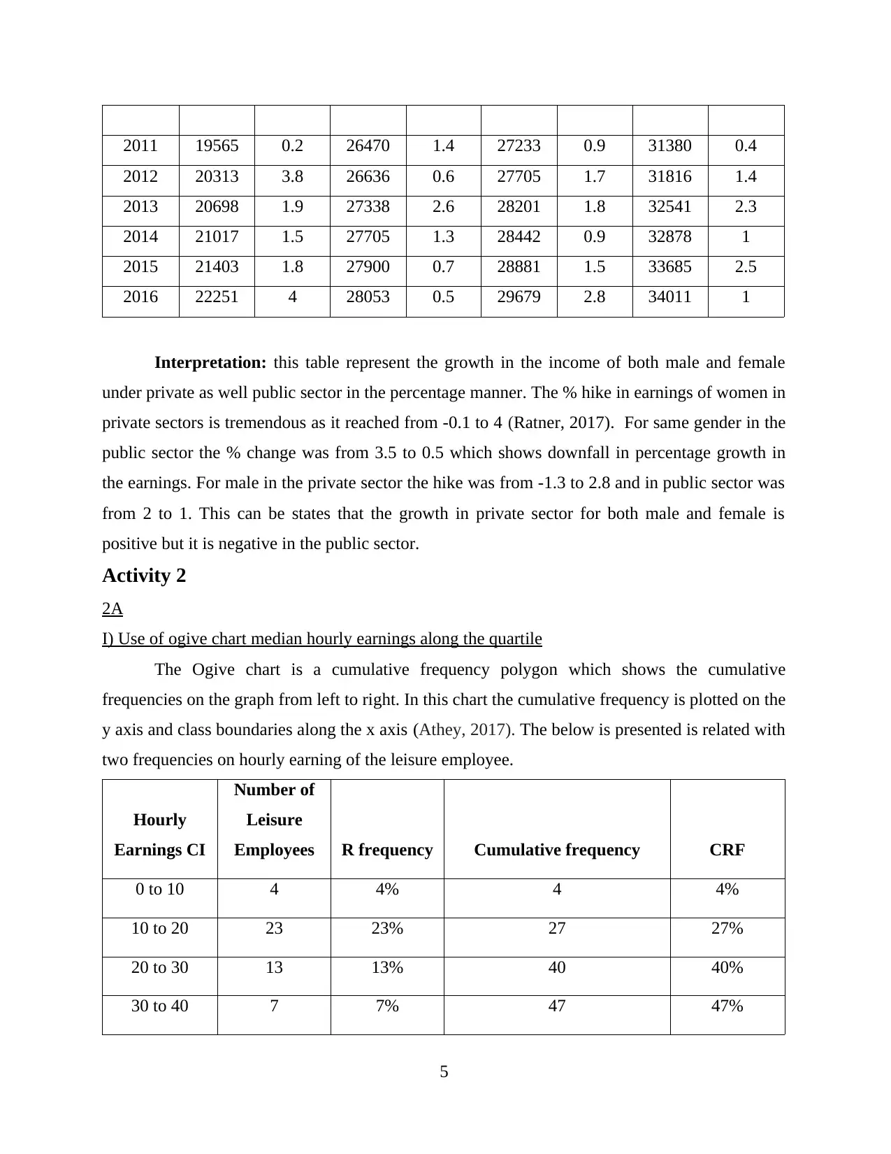
40 to 50 3 3% 50 50%
Hourly earnings Leisure Employees (F) Cumulative Frequency (Cf)
0 to 10 4 4
10 to 20 23 27
20 to 30 13 40
30 to 40 7 47
40 to 50 3 50
Median: L+ Cf-n/ f* I
20+(40-5)/ 50 * 10
27
Interpretation: the above O give graph represents the hourly earnings of the leisure
employee in the London. It can be seen that there is clear increase for the frequency level of 0-10
6
and 10-20 hours. From that till the 40-50 the CI is incising but the nuder of employee is
constantly decreasing.
The quartile of the above data depicts the fact that the observations are divided into 4
sections which are based on the value of data providing the difference in the whole observation
(Valickova, Havranek and Horvath,2015). It can be interpreted that the first quartile is at 25th
percentile, the second is at 50th percentile which is median value and third is at 75th percentile.
Range of Hourly Earnings (CI)
Number of Leisure Employees
(Frequency)
0 to 10 4
10 to 20 23
20 to 30 13
30 to 40 7
40 to 50 3
Quartile Outcome
1 4
2 7
3 13
Interpretation: it can be articulated from the above tabular calculation of the data that
the median value comes out to be 3 and the value in the 1st quartile have come as 4 which is not
near the median value. The value of 25th percentile is lower than then 25% and 75% quartile.
II) Calculation of the mean and standard deviation for hourly earnings
Mean value:
7
⊘ This is a preview!⊘
Do you want full access?
Subscribe today to unlock all pages.
Trusted by 1+ million students worldwide

Interpretation: The leisure employee are dented as F while the mid value is X with this
comes the total of employees and the frequency as FX. The total of the FX is dived by total of
the F which is calculated as 21.4. From this the values of FX is deducted and the resultant is
multiplied by itself to get its square (Kontopantelis and et.al., 2015). This can be simply stated
that total of FX that is 1070 is divided by 50 to get a mean value of 21.4.s
8
Paraphrase This Document
Need a fresh take? Get an instant paraphrase of this document with our AI Paraphraser
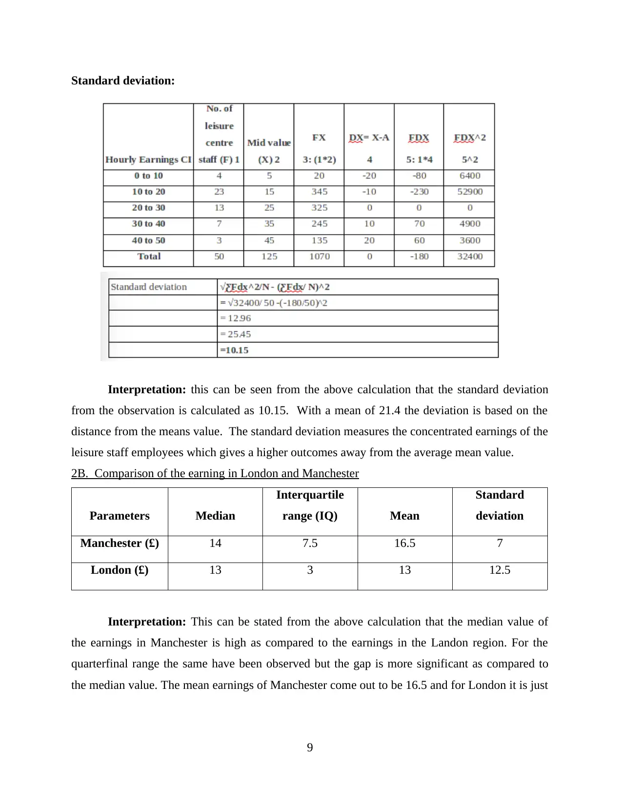
Standard deviation:
Interpretation: this can be seen from the above calculation that the standard deviation
from the observation is calculated as 10.15. With a mean of 21.4 the deviation is based on the
distance from the means value. The standard deviation measures the concentrated earnings of the
leisure staff employees which gives a higher outcomes away from the average mean value.
2B. Comparison of the earning in London and Manchester
Parameters Median
Interquartile
range (IQ) Mean
Standard
deviation
Manchester (£) 14 7.5 16.5 7
London (£) 13 3 13 12.5
Interpretation: This can be stated from the above calculation that the median value of
the earnings in Manchester is high as compared to the earnings in the Landon region. For the
quarterfinal range the same have been observed but the gap is more significant as compared to
the median value. The mean earnings of Manchester come out to be 16.5 and for London it is just
9

13. The deviation in the mean and the earnings is more in London. This depicts the facts the
earnings in the Manchester is far better than they are in the London region.
10
earnings in the Manchester is far better than they are in the London region.
10
⊘ This is a preview!⊘
Do you want full access?
Subscribe today to unlock all pages.
Trusted by 1+ million students worldwide
1 out of 15
Related Documents


Your All-in-One AI-Powered Toolkit for Academic Success.
+13062052269
info@desklib.com
Available 24*7 on WhatsApp / Email
![[object Object]](/_next/static/media/star-bottom.7253800d.svg)
Unlock your academic potential
Copyright © 2020–2026 A2Z Services. All Rights Reserved. Developed and managed by ZUCOL.