Probability, Hypothesis Testing, and Statistical Analysis
VerifiedAdded on 2020/05/28
|9
|1097
|250
AI Summary
The assignment delves into the application of statistical methods to real-world scenarios. It includes calculating probabilities for various events such as property price increases and customer service times, analyzing spending patterns using normal distribution, and conducting hypothesis tests to determine if there are significant differences in spending habits between genders.

Running head: STATISTICS FOR MANAGERIAL DECISIONS
Statistics for Managerial Decisions
Name of the student
Name of the university
Author’s note
Statistics for Managerial Decisions
Name of the student
Name of the university
Author’s note
Paraphrase This Document
Need a fresh take? Get an instant paraphrase of this document with our AI Paraphraser
1STATISTICS FOR MANAGERIAL DECISIONS
Table of Contents
Answer 1..........................................................................................................................................2
Part a............................................................................................................................................2
Part b............................................................................................................................................2
Part c............................................................................................................................................3
Answer 2..........................................................................................................................................3
Part a............................................................................................................................................3
Part b............................................................................................................................................3
Part c............................................................................................................................................4
Part d............................................................................................................................................4
Answer 3..........................................................................................................................................4
Part a............................................................................................................................................4
Part b............................................................................................................................................4
Part c............................................................................................................................................5
Part d............................................................................................................................................5
Answer 4..........................................................................................................................................5
Part a............................................................................................................................................5
Part b............................................................................................................................................6
Part c............................................................................................................................................6
Part i.........................................................................................................................................6
Part ii........................................................................................................................................6
Answer 5..........................................................................................................................................6
Part a............................................................................................................................................6
Part b............................................................................................................................................7
Part c............................................................................................................................................7
2STATISTICS FOR MANAGERIAL DECISIONS
Answer 1
Part a
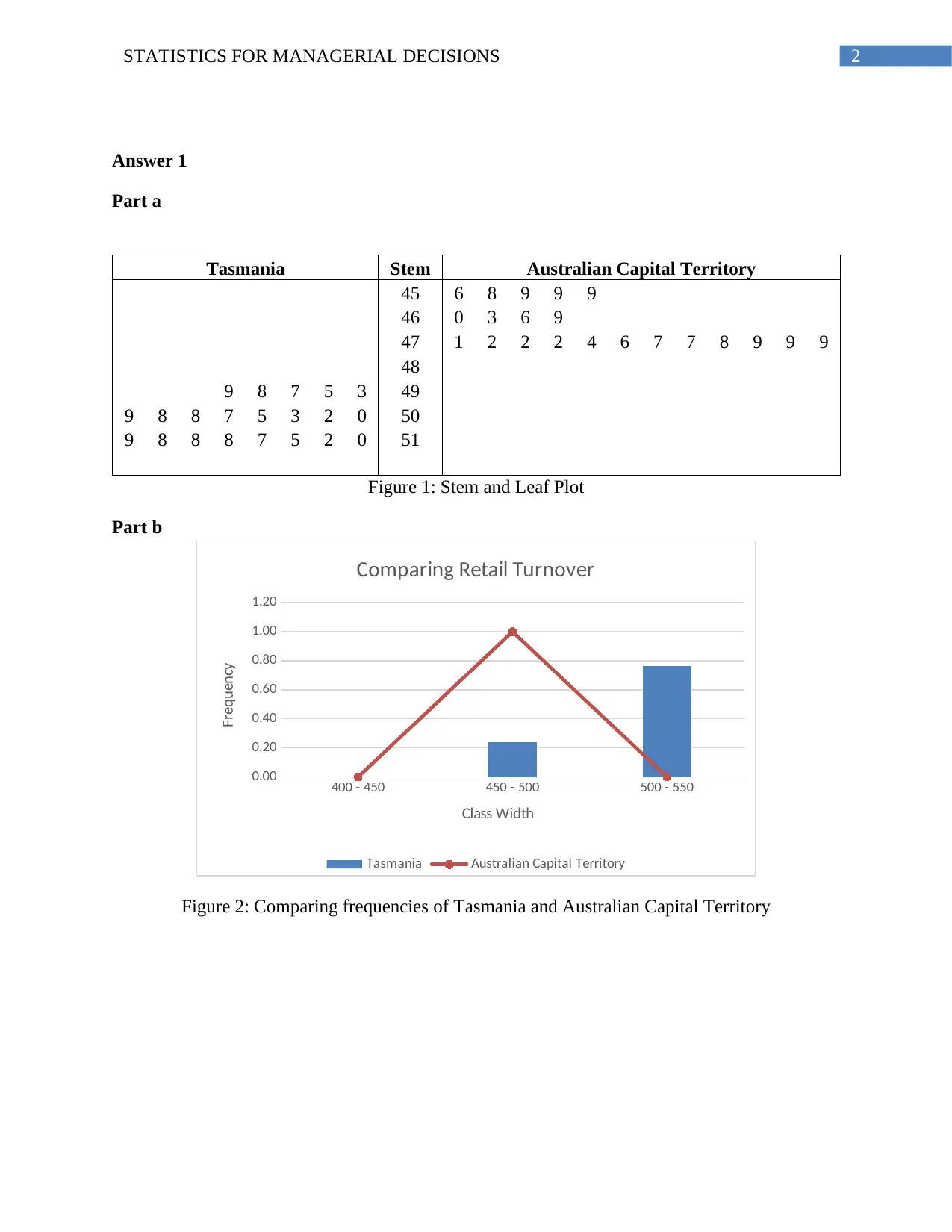
Tasmania Stem Australian Capital Territory
45 6 8 9 9 9
46 0 3 6 9
47 1 2 2 2 4 6 7 7 8 9 9 9
48
9 8 7 5 3 49
9 8 8 7 5 3 2 0 50
9 8 8 8 7 5 2 0 51
Figure 1: Stem and Leaf Plot
Part b
400 - 450 450 - 500 500 - 550
0.00
0.20
0.40
0.60
0.80
1.00
1.20
Comparing Retail Turnover
Tasmania Australian Capital Territory
Class Width
Frequency
Figure 2: Comparing frequencies of Tasmania and Australian Capital Territory
Answer 1
Part a
Tasmania Stem Australian Capital Territory
45 6 8 9 9 9
46 0 3 6 9
47 1 2 2 2 4 6 7 7 8 9 9 9
48
9 8 7 5 3 49
9 8 8 7 5 3 2 0 50
9 8 8 8 7 5 2 0 51
Figure 1: Stem and Leaf Plot
Part b
400 - 450 450 - 500 500 - 550
0.00
0.20
0.40
0.60
0.80
1.00
1.20
Comparing Retail Turnover
Tasmania Australian Capital Territory
Class Width
Frequency
Figure 2: Comparing frequencies of Tasmania and Australian Capital Territory
⊘ This is a preview!⊘
Do you want full access?
Subscribe today to unlock all pages.
Trusted by 1+ million students worldwide
3STATISTICS FOR MANAGERIAL DECISIONS
Part c
Jan-16
Feb-16
Mar-16
Apr-16
May-16
Jun-16
Jul-16
Aug-16
Sep-16
Oct-16
Nov-16
Dec-16
Jan-17
Feb-17
Mar-17
Apr-17
May-17
Jun-17
Jul-17
Aug-17
Sep-17
420
440
460
480
500
520
540
Comparing Retail Turnover
Tasmania Australian Capital Territory
Timeline
Retail Values ($million)
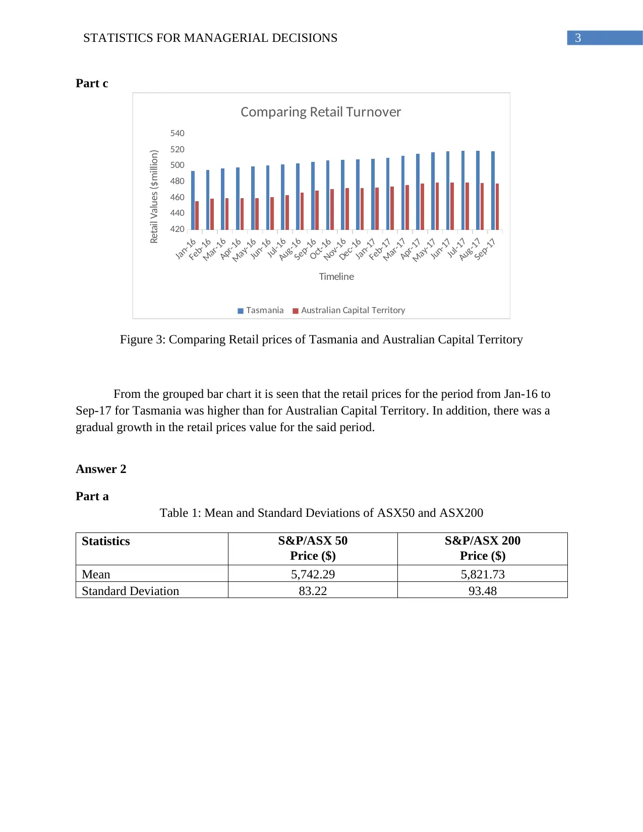
Figure 3: Comparing Retail prices of Tasmania and Australian Capital Territory
From the grouped bar chart it is seen that the retail prices for the period from Jan-16 to
Sep-17 for Tasmania was higher than for Australian Capital Territory. In addition, there was a
gradual growth in the retail prices value for the said period.
Answer 2
Part a
Table 1: Mean and Standard Deviations of ASX50 and ASX200
Statistics S&P/ASX 50 S&P/ASX 200
Price ($) Price ($)
Mean 5,742.29 5,821.73
Standard Deviation 83.22 93.48
Part c
Jan-16
Feb-16
Mar-16
Apr-16
May-16
Jun-16
Jul-16
Aug-16
Sep-16
Oct-16
Nov-16
Dec-16
Jan-17
Feb-17
Mar-17
Apr-17
May-17
Jun-17
Jul-17
Aug-17
Sep-17
420
440
460
480
500
520
540
Comparing Retail Turnover
Tasmania Australian Capital Territory
Timeline
Retail Values ($million)
Figure 3: Comparing Retail prices of Tasmania and Australian Capital Territory
From the grouped bar chart it is seen that the retail prices for the period from Jan-16 to
Sep-17 for Tasmania was higher than for Australian Capital Territory. In addition, there was a
gradual growth in the retail prices value for the said period.
Answer 2
Part a
Table 1: Mean and Standard Deviations of ASX50 and ASX200
Statistics S&P/ASX 50 S&P/ASX 200
Price ($) Price ($)
Mean 5,742.29 5,821.73
Standard Deviation 83.22 93.48
Paraphrase This Document
Need a fresh take? Get an instant paraphrase of this document with our AI Paraphraser
4STATISTICS FOR MANAGERIAL DECISIONS
Part b
Table 2: Statistics for ASX50 and ASX200
Statistics S&P/ASX 50 S&P/ASX 200
Price ($) Price ($)
Minimum 5,584.02 5,651.77
Q1 5669.215 5738.3975
Median 5,786.52 5,868.19
Q3 5810.1775 5901.7725
Maximum 5,825.99 5,919.08
Part c
S&P/ASX 50 S&P/ASX 200
5500
5550
5600
5650
5700
5750
5800
5850
5900
5950
Box and Whisker plot of the share prices
Shares
Prices ($)
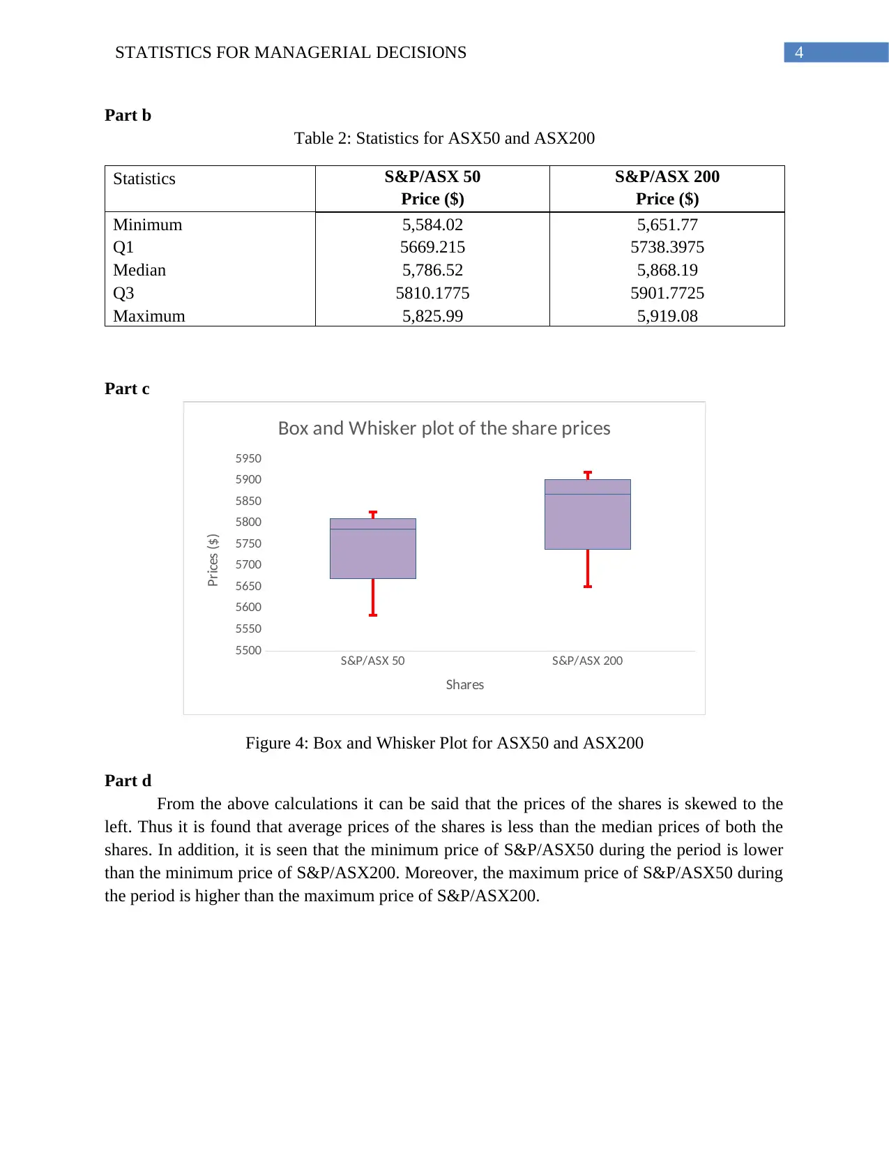
Figure 4: Box and Whisker Plot for ASX50 and ASX200
Part d
From the above calculations it can be said that the prices of the shares is skewed to the
left. Thus it is found that average prices of the shares is less than the median prices of both the
shares. In addition, it is seen that the minimum price of S&P/ASX50 during the period is lower
than the minimum price of S&P/ASX200. Moreover, the maximum price of S&P/ASX50 during
the period is higher than the maximum price of S&P/ASX200.
Part b
Table 2: Statistics for ASX50 and ASX200
Statistics S&P/ASX 50 S&P/ASX 200
Price ($) Price ($)
Minimum 5,584.02 5,651.77
Q1 5669.215 5738.3975
Median 5,786.52 5,868.19
Q3 5810.1775 5901.7725
Maximum 5,825.99 5,919.08
Part c
S&P/ASX 50 S&P/ASX 200
5500
5550
5600
5650
5700
5750
5800
5850
5900
5950
Box and Whisker plot of the share prices
Shares
Prices ($)
Figure 4: Box and Whisker Plot for ASX50 and ASX200
Part d
From the above calculations it can be said that the prices of the shares is skewed to the
left. Thus it is found that average prices of the shares is less than the median prices of both the
shares. In addition, it is seen that the minimum price of S&P/ASX50 during the period is lower
than the minimum price of S&P/ASX200. Moreover, the maximum price of S&P/ASX50 during
the period is higher than the maximum price of S&P/ASX200.
5STATISTICS FOR MANAGERIAL DECISIONS
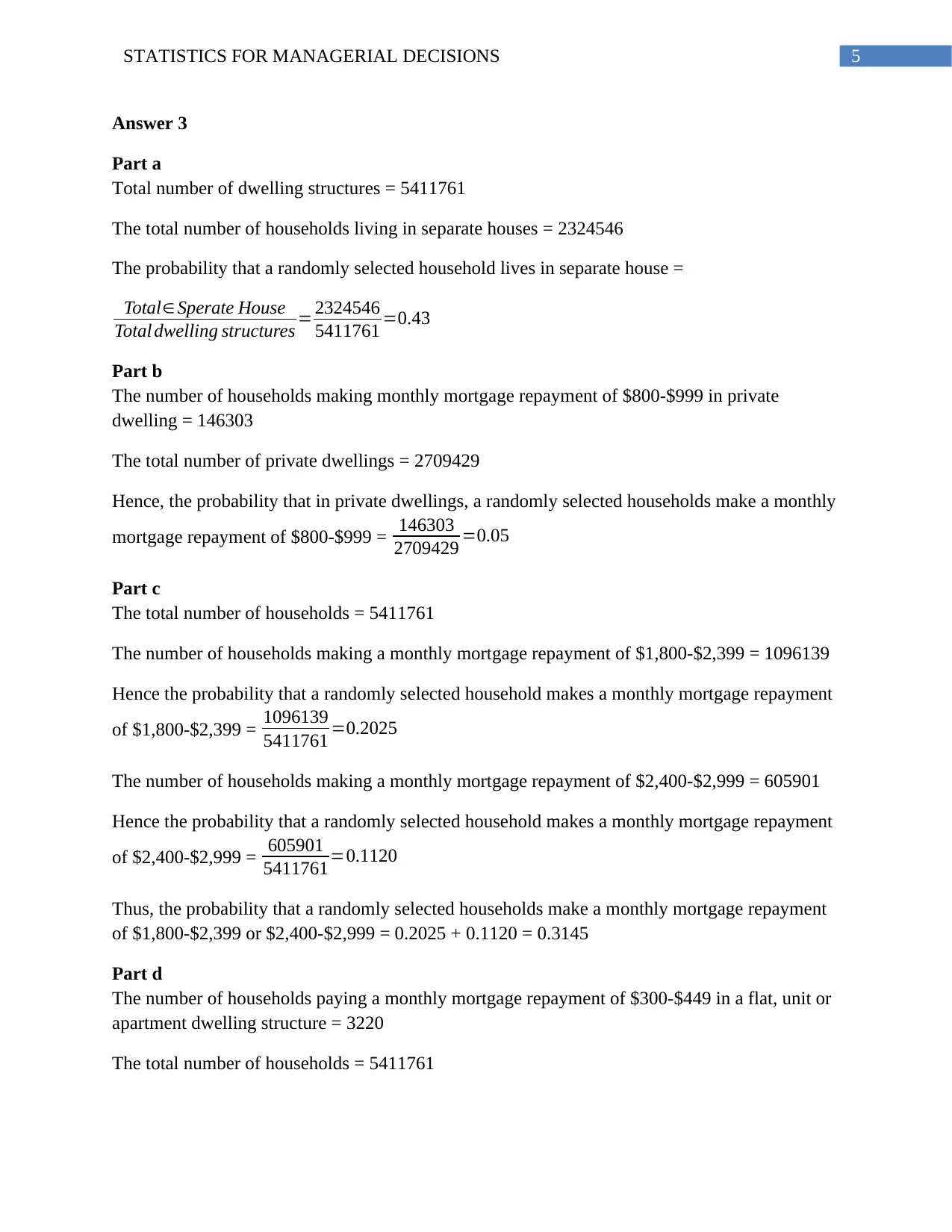
Answer 3
Part a
Total number of dwelling structures = 5411761
The total number of households living in separate houses = 2324546
The probability that a randomly selected household lives in separate house =
Total∈Sperate House
Total dwelling structures = 2324546
5411761 =0.43
Part b
The number of households making monthly mortgage repayment of $800-$999 in private
dwelling = 146303
The total number of private dwellings = 2709429
Hence, the probability that in private dwellings, a randomly selected households make a monthly
mortgage repayment of $800-$999 = 146303
2709429 =0.05
Part c
The total number of households = 5411761
The number of households making a monthly mortgage repayment of $1,800-$2,399 = 1096139
Hence the probability that a randomly selected household makes a monthly mortgage repayment
of $1,800-$2,399 = 1096139
5411761 =0.2025
The number of households making a monthly mortgage repayment of $2,400-$2,999 = 605901
Hence the probability that a randomly selected household makes a monthly mortgage repayment
of $2,400-$2,999 = 605901
5411761=0.1120
Thus, the probability that a randomly selected households make a monthly mortgage repayment
of $1,800-$2,399 or $2,400-$2,999 = 0.2025 + 0.1120 = 0.3145
Part d
The number of households paying a monthly mortgage repayment of $300-$449 in a flat, unit or
apartment dwelling structure = 3220
The total number of households = 5411761
⊘ This is a preview!⊘
Do you want full access?
Subscribe today to unlock all pages.
Trusted by 1+ million students worldwide
6STATISTICS FOR MANAGERIAL DECISIONS
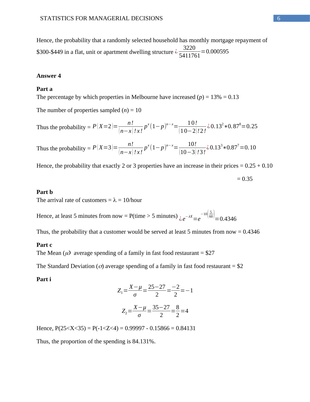
Hence, the probability that a randomly selected household has monthly mortgage repayment of
$300-$449 in a flat, unit or apartment dwelling structure ¿ 3220
5411761=0.000595
Answer 4
Part a
The percentage by which properties in Melbourne have increased (p) = 13% = 0.13
The number of properties sampled (n) = 10
Thus the probability = P ( X=2 ) = n !
( n−x ) ! x ! px (1− p)n− x= 1 0 !
( 1 0−2 ) ! 2 ! ¿ 0.132∗0. 878=0.25
Thus the probability = P ( X=3 ) = n!
( n−x ) ! x ! px (1− p)n− x= 10!
( 10−3 ) ! 3 ! ¿ 0.133∗0.877 =0. 10
Hence, the probability that exactly 2 or 3 properties have an increase in their prices = 0.25 + 0.10
= 0.35
Part b
The arrival rate of customers = = 10/hour
Hence, at least 5 minutes from now = P(time > 5 minutes) ¿ e− λX =e−10 ( 5
60 )=0.4346
Thus, the probability that a customer would be served at least 5 minutes from now = 0.4346
Part c
The Mean (
average spending of a family in fast food restaurant = $27
The Standard Deviation (
) average spending of a family in fast food restaurant = $2
Part i
Z1 = X−μ
σ = 25−27
2 =−2
2 =−1
Z2 = X−μ
σ = 35−27
2 =8
2 =4
Hence, P(25<X<35) = P(-1<Z<4) = 0.99997 - 0.15866 = 0.84131
Thus, the proportion of the spending is 84.131%.
Paraphrase This Document
Need a fresh take? Get an instant paraphrase of this document with our AI Paraphraser
7STATISTICS FOR MANAGERIAL DECISIONS
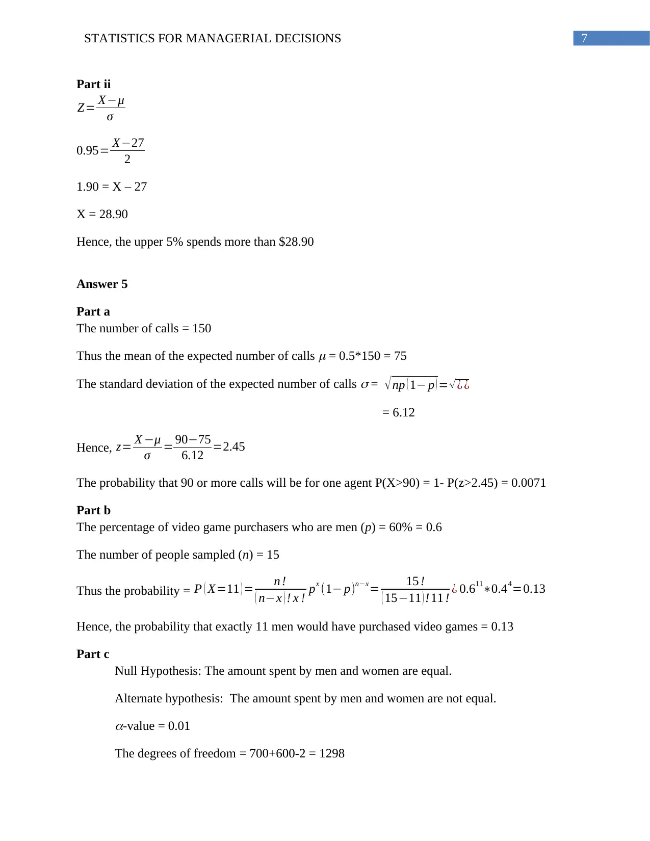
Part ii
Z= X−μ
σ
0.95= X−27
2
1.90 = X – 27
X = 28.90
Hence, the upper 5% spends more than $28.90
Answer 5
Part a
The number of calls = 150
Thus the mean of the expected number of calls
= 0.5*150 = 75
The standard deviation of the expected number of calls
= √ np ( 1− p ) = √ ¿ ¿
= 6.12
Hence, z= X −μ
σ = 90−75
6.12 =2.45
The probability that 90 or more calls will be for one agent P(X>90) = 1- P(z>2.45) = 0.0071
Part b
The percentage of video game purchasers who are men (p) = 60% = 0.6
The number of people sampled (n) = 15
Thus the probability = P ( X=11 ) = n !
( n−x ) ! x ! px (1− p)n−x= 15 !
( 15−11 ) ! 11 ! ¿ 0.611∗0.44=0.13
Hence, the probability that exactly 11 men would have purchased video games = 0.13
Part c
Null Hypothesis: The amount spent by men and women are equal.
Alternate hypothesis: The amount spent by men and women are not equal.-value = 0.01
The degrees of freedom = 700+600-2 = 1298
8STATISTICS FOR MANAGERIAL DECISIONS
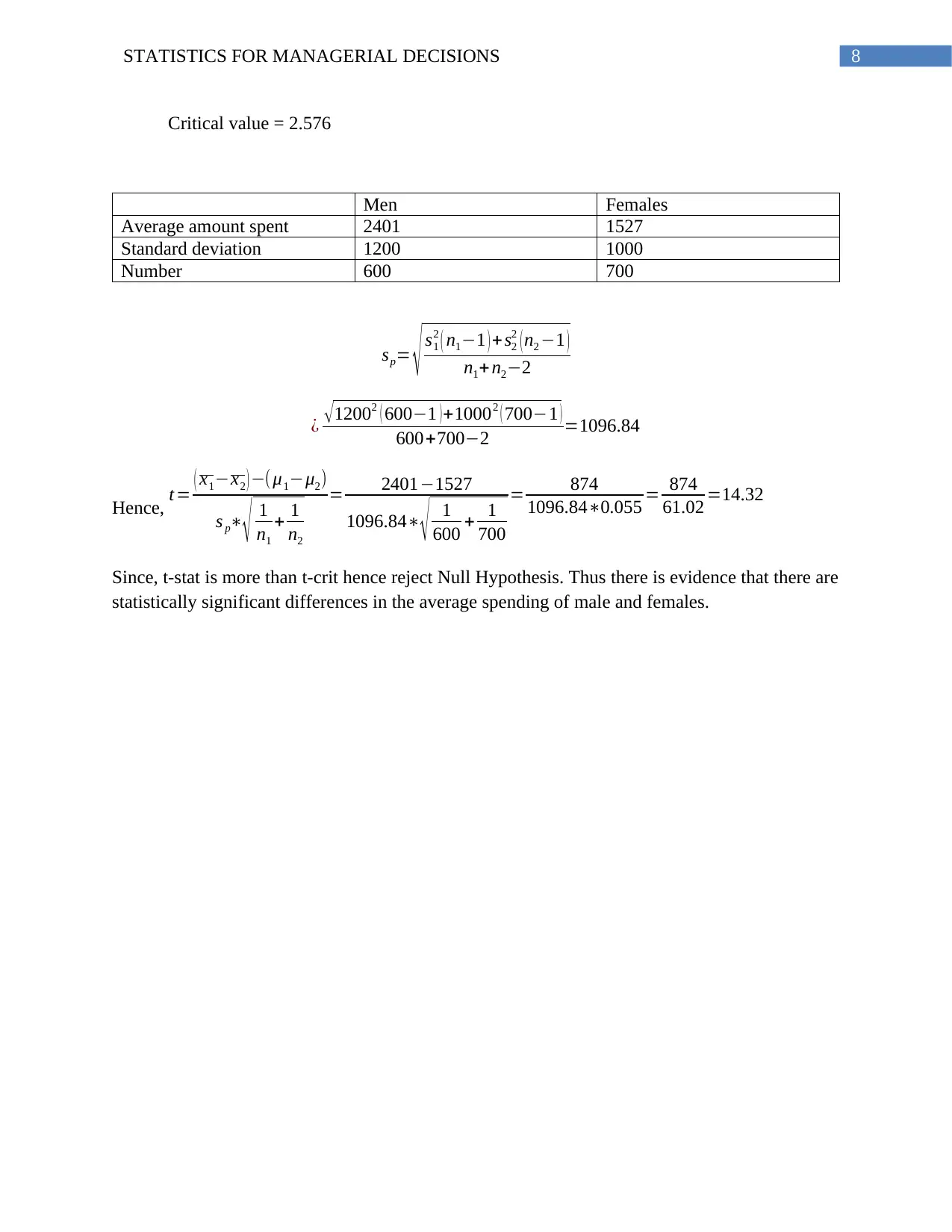
Critical value = 2.576
Men Females
Average amount spent 2401 1527
Standard deviation 1200 1000
Number 600 700
sp= √ s1
2 ( n1−1 ) + s2
2 (n2 −1 )
n1+ n2−2
¿ √12002 ( 600−1 )+10002 ( 700−1 )
600+700−2 =1096.84
Hence, t= ( x1−x2 ) −(μ1−μ2)
s p∗
√ 1
n1
+ 1
n2
= 2401−1527
1096.84∗
√ 1
600 + 1
700
= 874
1096.84∗0.055 = 874
61.02 =14.32
Since, t-stat is more than t-crit hence reject Null Hypothesis. Thus there is evidence that there are
statistically significant differences in the average spending of male and females.
⊘ This is a preview!⊘
Do you want full access?
Subscribe today to unlock all pages.
Trusted by 1+ million students worldwide
1 out of 9
Related Documents


Your All-in-One AI-Powered Toolkit for Academic Success.
+13062052269
info@desklib.com
Available 24*7 on WhatsApp / Email
![[object Object]](/_next/static/media/star-bottom.7253800d.svg)
Unlock your academic potential
Copyright © 2020–2026 A2Z Services. All Rights Reserved. Developed and managed by ZUCOL.