Statistical Tests: t-Test, U-Test, ANOVA, and Kruskal-Wallis Analysis

This assignment delves into various statistical tests, including the independent samples t-test, Mann-Whitney U-test, paired t-test, Wilcoxon Matched-Pairs Signed Rank Test, One-Way ANOVA, and Kruskal-Wallis H-Test. Students are tasked with understanding the assumptions of each test, formulating research questions and hypotheses, generating datasets, performing analyses using SPSS, and interpreting the results. The assignment requires the computation of descriptive statistics, the application of appropriate statistical procedures, and the determination of statistical significance to draw conclusions. It covers both parametric and non-parametric tests, offering a comprehensive overview of statistical analysis techniques. The analysis involves interpretation of SPSS outputs and drawing conclusions based on the p-values obtained. The assignment emphasizes the importance of understanding the assumptions of each test and selecting the appropriate test based on the nature of the data and research question.

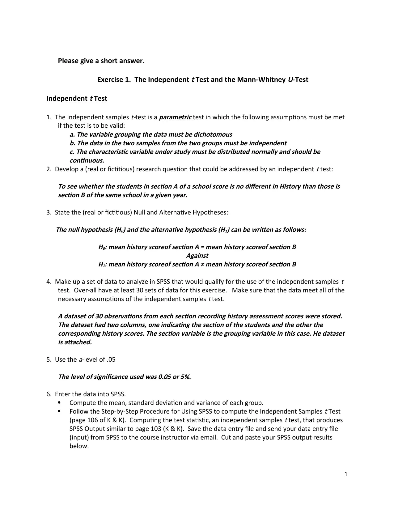
Please give a short answer.
Exercise 1. The Independent
t Test and the Mann-Whitney
U-Test
Independent
t Test
1. The independent samples
t-test is a
parametric test in which the following assumptions must be met
if the test is to be valid:
a. The variable grouping the data must be dichotomous
b. The data in the two samples from the two groups must be independent
c. The characteristic variable under study must be distributed normally and should be
continuous.
2. Develop a (real or fictitious) research question that could be addressed by an independent
t test:To see whether the students in section A of a school score is no different in History than those is
section B of the same school in a given year.
3. State the (real or fictitious) Null and Alternative Hypotheses:The null hypothesis (H0) and the alternative hypothesis (H1) can be written as follows:
H0: mean history scoreof section A = mean history scoreof section B
Against
H1: mean history scoreof section A ≠ mean history scoreof section B
4. Make up a set of data to analyze in SPSS that would qualify for the use of the independent samples
t
test. Over-all have at least 30 sets of data for this exercise. Make sure that the data meet all of the
necessary assumptions of the independent samples
t test.A dataset of 30 observations from each section recording history assessment scores were stored.
The dataset had two columns, one indicating the section of the students and the other the
corresponding history scores. The section variable is the grouping variable in this case. He dataset
is attached.
5. Use the
a-level of .05The level of significance used was 0.05 or 5%.
6. Enter the data into SPSS.
 Compute the mean, standard deviation and variance of each group.
 Follow the Step-by-Step Procedure for Using SPSS to compute the Independent Samples
t Test
(page 106 of K & K). Computing the test statistic, an independent samples
t test, that produces
SPSS Output similar to page 103 (K & K). Save the data entry file and send your data entry file
(input) from SPSS to the course instructor via email. Cut and paste your SPSS output results
below.
1

The SPSS output showing the necessary computations are given hence:
Group Statistics
Section N Mean Std. Deviation Std. Error Mean
Marks Section A 30 46.4667 28.36673 5.17903
Section B 30 57.8667 30.14875 5.50438
Independent Samples Test
Levene's Test
for Equality of
Variances
t-test for Equality of Means
F Sig. t df Sig. (2-
tailed)
Mean
Difference
Std. Error
Difference
95% Confidence
Interval of the
Difference
Lower Upper
Marks
Equal
variances
assumed
.114 .736 -
1.508 58 .137 -11.40000 7.55782 -26.52862 3.72862
Equal
variances
not assumed
-
1.508 57.786 .137 -11.40000 7.55782 -26.52981 3.72981
7. Determine the Statistical Significance and State a Conclusion. (Use the example “Putting it All
Together” on page 107 (K & K)The statistical level of significance is 0.137 which is greater than the a-level which is 0.05.
Therefore the test is not significant and the test fails to reject null hypothesis. Hence there is not
enough evidence to support the conjecture that section A has better or worse scores than section
B.
Mann-Whitney
U-Test
1. The Mann-Whitney
U-Test is a
non-parametrictest in which the following assumptions must be met if
the test is to be valid:a.The grouping variable must be dichotomous
2

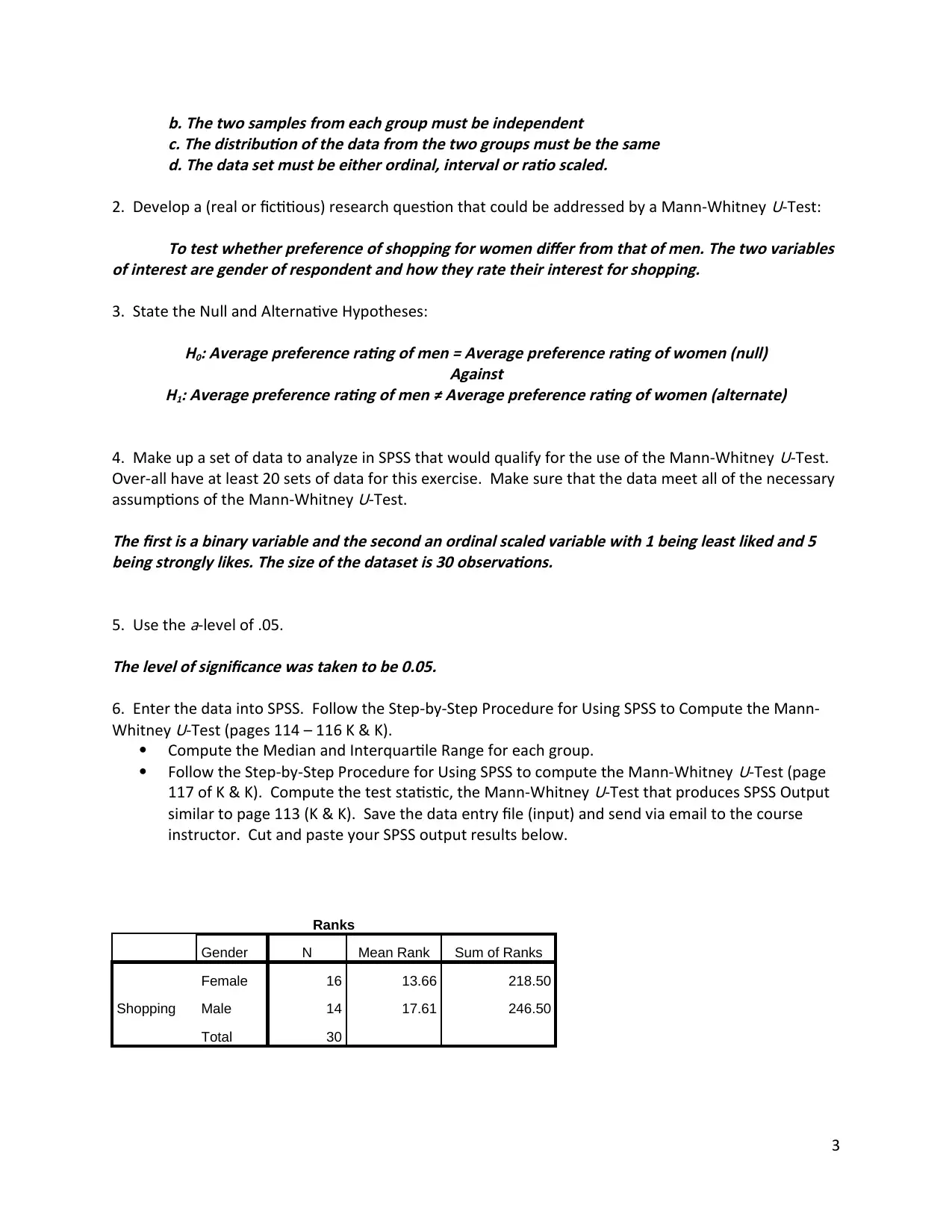
b. The two samples from each group must be independent
c. The distribution of the data from the two groups must be the same
d. The data set must be either ordinal, interval or ratio scaled.
2. Develop a (real or fictitious) research question that could be addressed by a Mann-Whitney
U-Test:To test whether preference of shopping for women differ from that of men. The two variables
of interest are gender of respondent and how they rate their interest for shopping.
3. State the Null and Alternative Hypotheses:H0: Average preference rating of men = Average preference rating of women (null)
Against
H1: Average preference rating of men ≠ Average preference rating of women (alternate)
4. Make up a set of data to analyze in SPSS that would qualify for the use of the Mann-Whitney
U-Test.
Over-all have at least 20 sets of data for this exercise. Make sure that the data meet all of the necessary
assumptions of the Mann-Whitney
U-Test.
The first is a binary variable and the second an ordinal scaled variable with 1 being least liked and 5
being strongly likes. The size of the dataset is 30 observations.
5. Use the
a-level of .05.
The level of significance was taken to be 0.05.
6. Enter the data into SPSS. Follow the Step-by-Step Procedure for Using SPSS to Compute the Mann-
Whitney
U-Test (pages 114 – 116 K & K).
 Compute the Median and Interquartile Range for each group.
 Follow the Step-by-Step Procedure for Using SPSS to compute the Mann-Whitney
U-Test (page
117 of K & K). Compute the test statistic, the Mann-Whitney
U-Test that produces SPSS Output
similar to page 113 (K & K). Save the data entry file (input) and send via email to the course
instructor. Cut and paste your SPSS output results below.
Ranks
Gender N Mean Rank Sum of Ranks
Shopping
Female 16 13.66 218.50
Male 14 17.61 246.50
Total 30
3

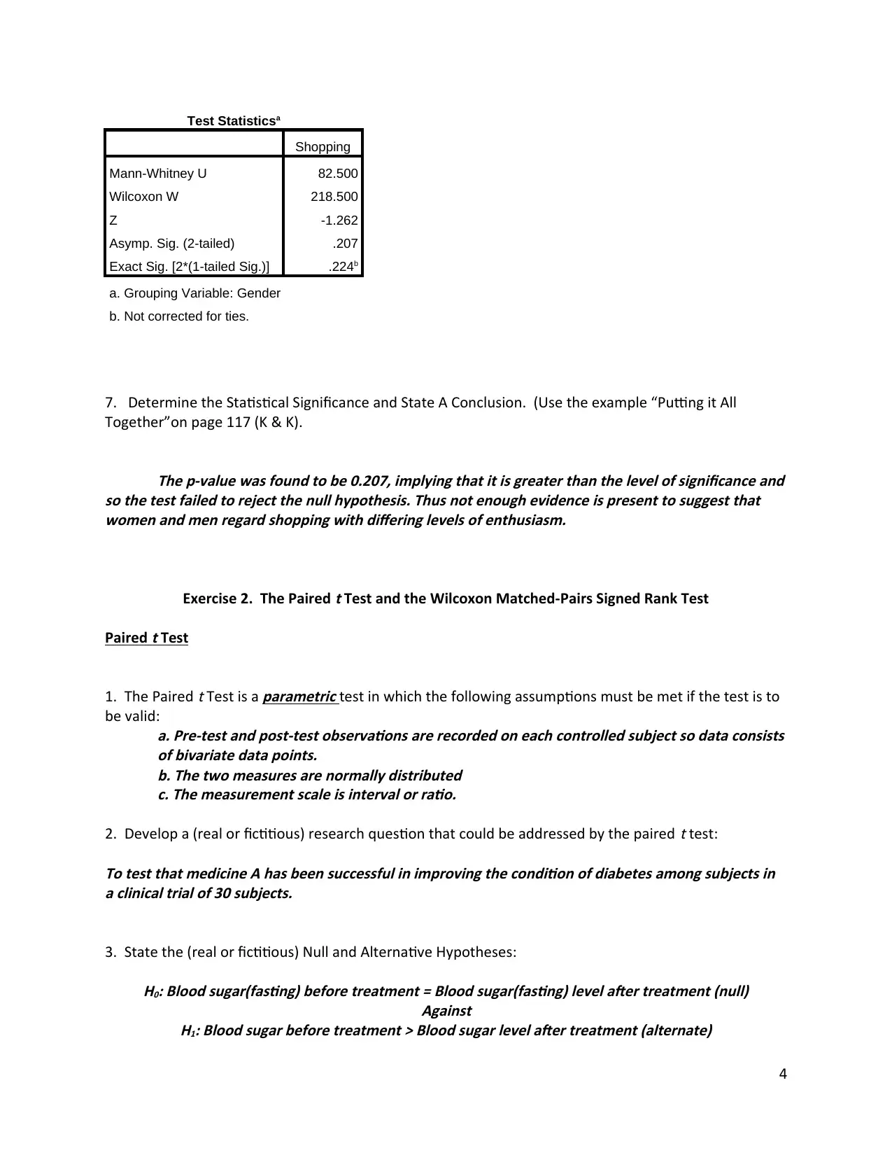
Test Statisticsa
Shopping
Mann-Whitney U 82.500
Wilcoxon W 218.500
Z -1.262
Asymp. Sig. (2-tailed) .207
Exact Sig. [2*(1-tailed Sig.)] .224b
a. Grouping Variable: Gender
b. Not corrected for ties.
7. Determine the Statistical Significance and State A Conclusion. (Use the example “Putting it All
Together”on page 117 (K & K).
The p-value was found to be 0.207, implying that it is greater than the level of significance and
so the test failed to reject the null hypothesis. Thus not enough evidence is present to suggest that
women and men regard shopping with differing levels of enthusiasm.
Exercise 2. The Paired
t Test and the Wilcoxon Matched-Pairs Signed Rank Test
Paired
t Test
1. The Paired
t Test is a
parametric test in which the following assumptions must be met if the test is to
be valid:
a. Pre-test and post-test observations are recorded on each controlled subject so data consists
of bivariate data points.
b. The two measures are normally distributed
c. The measurement scale is interval or ratio.
2. Develop a (real or fictitious) research question that could be addressed by the paired
t test:
To test that medicine A has been successful in improving the condition of diabetes among subjects in
a clinical trial of 30 subjects.
3. State the (real or fictitious) Null and Alternative Hypotheses:H0: Blood sugar(fasting) before treatment = Blood sugar(fasting) level after treatment (null)
Against
H1: Blood sugar before treatment > Blood sugar level after treatment (alternate)
4

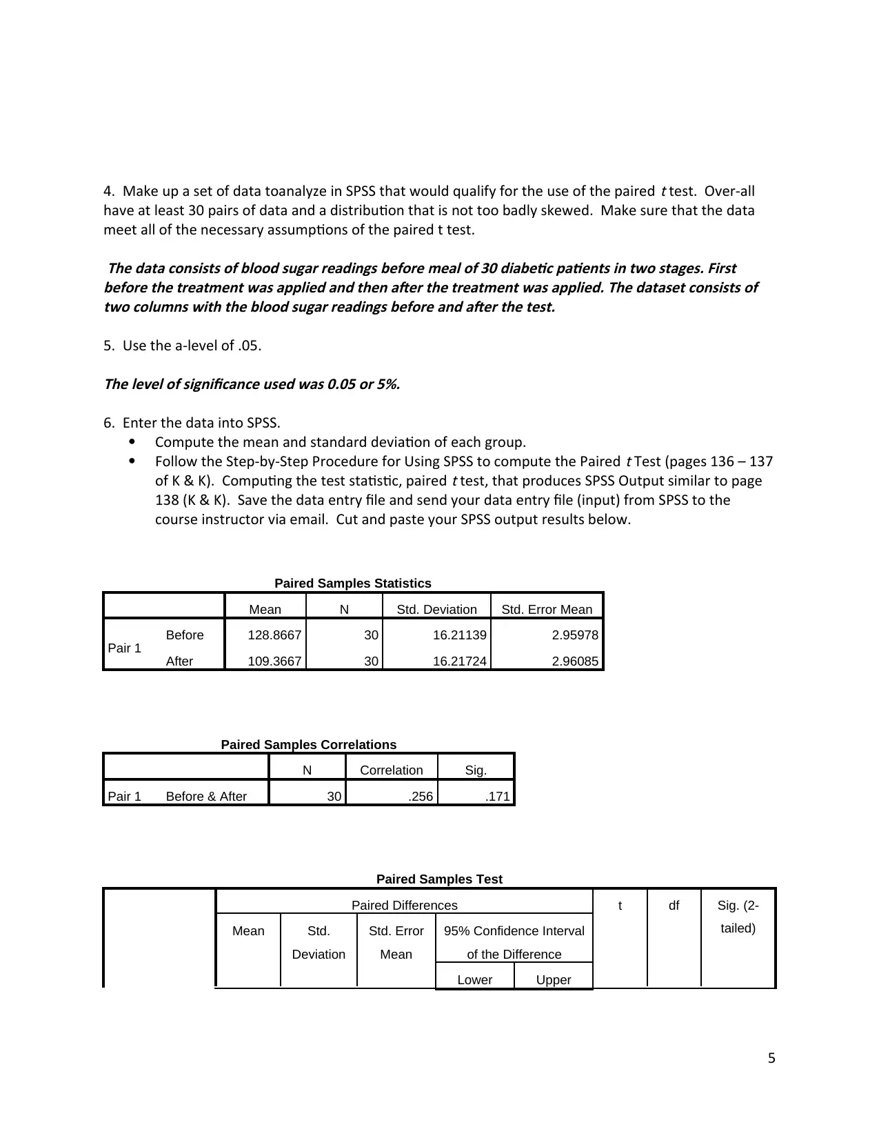
4. Make up a set of data toanalyze in SPSS that would qualify for the use of the paired
t test. Over-all
have at least 30 pairs of data and a distribution that is not too badly skewed. Make sure that the data
meet all of the necessary assumptions of the paired t test.
The data consists of blood sugar readings before meal of 30 diabetic patients in two stages. First
before the treatment was applied and then after the treatment was applied. The dataset consists of
two columns with the blood sugar readings before and after the test.
5. Use the a-level of .05.
The level of significance used was 0.05 or 5%.
6. Enter the data into SPSS.
 Compute the mean and standard deviation of each group.
 Follow the Step-by-Step Procedure for Using SPSS to compute the Paired
t Test (pages 136 – 137
of K & K). Computing the test statistic, paired
t test, that produces SPSS Output similar to page
138 (K & K). Save the data entry file and send your data entry file (input) from SPSS to the
course instructor via email. Cut and paste your SPSS output results below.
Paired Samples Statistics
Mean N Std. Deviation Std. Error Mean
Pair 1 Before 128.8667 30 16.21139 2.95978
After 109.3667 30 16.21724 2.96085
Paired Samples Correlations
N Correlation Sig.
Pair 1 Before & After 30 .256 .171
Paired Samples Test
Paired Differences t df Sig. (2-
tailed)Mean Std.
Deviation
Std. Error
Mean
95% Confidence Interval
of the Difference
Lower Upper
5

Pair
1
Before -
After 19.50000 19.77241 3.60993 12.11686 26.88314 5.402 29 .000
7. Determine the Statistical Significance and State a Conclusion. (Use the example “Putting it All
Together” on page 138 (K & K)).The p-value was found to be less than 0.0001 and hence much lower than the level of
significance assumed which is 0.05. Thus the test rejected the null hypothesis at 5% level of
significance.
Wilcoxon Matched-Pairs Test
Review pages 137 - 144 in Kellar & Kelvin (K & K).
1. The Wilcoxon Matched-Pairs Test is a test in which the following assumptions must be met if the test
is to be valid:a. Pre-test and post-test observations are recorded on each controlled subject so data consists
of bivariate data points.
b. The two measures follow the same distribution.
c. The measurement scale is ordered, interval or ratio.
2. Develop a (real or fictitious) research question that could be addressed by the Wilcoxon Matched-
Pairs Test:
To check whether a treatment plan for treating joint pains in athletes was successful in reducing pain
or not.
3. State the (real or fictitious) Null and Alternative Hypotheses:
H0: Pain level before treatment = Pain level after treatment (null)
Against
H1: Pain level before treatment > Pain level after treatment (alternate)
4. Make up a set of data to analyze in SPSS that would qualify for the use of the Wilcoxon Matched-
Pairs Test. Over-all have at least 20 pairs of data. Make sure that the data meet all of the necessary
assumptions of the Wilcoxon Matched-Pairs Test.
The pain levels of 30 athletes suffering from acute joint pain who were undergoing the treatment was
recorded before and after the treatment in two separate columns. The pain level was recorded in a
scale of 1 to 10 with 1 being least and 10 being strong pain.
6

5. Use the a-level of .05.
The level of significance used was 0.05 or 5%.
6. Enter the data into SPSS.
 Compute the median and interquartile range for each group.
 Follow the Step-by-Step Procedure for Using SPSS to compute the Wilcoxon Matched-Pairs
Statistics (page 144 of K & K). Computing the test statistic, Wilcoxon Matched-Pairs, that
produces SPSS Output similar to page 143 (K & K). Save the data entry file and send your data
entry file (input) from SPSS to the course instructor via email. Cut and paste your SPSS output
results below.
Ranks
N Mean Rank Sum of Ranks
PainAfter - PainBefore
Negative Ranks 20a 15.68 313.50
Positive Ranks 6b 6.25 37.50
Ties 4c
Total 30
a. PainAfter < PainBefore
b. PainAfter > PainBefore
c. PainAfter = PainBefore
Test Statisticsa
PainAfter -
PainBefore
Z -3.531b
Asymp. Sig. (2-tailed) .000
a. Wilcoxon Signed Ranks Test
b. Based on positive ranks.
7. Determine the Statistical Significance and State a Conclusion. (Use the example “Putting it All
Together” on page 144 (K & K)).The p-vale was found to be less than 0.0001 and hence much lower than the value of
significance 0.05. Therefore the null is to be rejected at 5% level and it suggests that the treatment did
indeed reduce pain in the patients.
7

Exercise 3. The One-Way ANOVA and the Kruskal-Wallis
H-Test
The One-Way ANOVA
Review pages 151 – 171in Kellar & Kelvin (K & K).
1. The One-Way ANOVA is a
parametric test in which the following assumptions must be met if the test
is to be valid:a. The sample of data of interest is an independent random sample.
b. The grouping variable has more than 2 categories.
c. The measure of the data of interest is distributed normally.
d. The variable is measured in either interval or ratio scale.
e. The variance is homogeneous among all of the groups.
2. List and define each of the commonly used post hoc tests for analysis of variance models.a.Least significance difference test is equivalent to multiple t-tests where the pooled estimate
of the variance is employed instead of comparing the variance which are common to all
groups.
b.Scheffe Test is based on the formula for t-test or f-ratio test. The critical value determines
whether the resulting F statistic is significant or not.
c.Tukey’s Honestly Significant Difference is the least powerful test of all the others defined
here. The critical values remain the same for all comparisons irrespective of the number of
mean comparisons.
d.Student Newman-Keuls test is similar to Tukey’s HSD but the critical values do not stay
equal and reflect the variable which are being compared.
e.Duncan Test is compared in the same way as Student Newman Keuls however in this case
the critical value is not at stringent as the latter.
f. Bonferroni Correction divides the alpha level by the number of comparisons of groups that
are to be made and the test for significance is carried out accordingly.
g.Tukey’s wholly significant difference makes use of critical values which are the average of
that in Tukey’s HSD and Student Newman-keuls. It is a moderated measure between the two.
3. Develop a (real or fictitious) research question that could be addressed by a One-Way ANOVA:To test whether the scores in Math of students in the tenth grade differs among schools from
three districts A, B, C.
4. State the (real or fictitious) Null and Alternative Hypotheses:
H0: Average math score is equal for all districts A, B, C (null)
Against
H1: At least one inequality among the math scores exists over the districts (alternate)
5. Make up a set of data to analyze in SPSS that would qualify for the use of the One-Way ANOVA.
Over-all have at least 30 data points in each of the three groups for this exercise. Make sure that data
8

meet all of the necessary assumptions of the One-Way ANOVA. If necessary for your final results, pick
and use the appropriate post hoc test.The data consists of average school math scores from 45 schools from over 3 districts A, B and
C. The two variables district and score shows the district from which the data point has been recorded
and the average score of the school in math.
6. State your a-level:
The level of significance used was 0.05 or 5%.
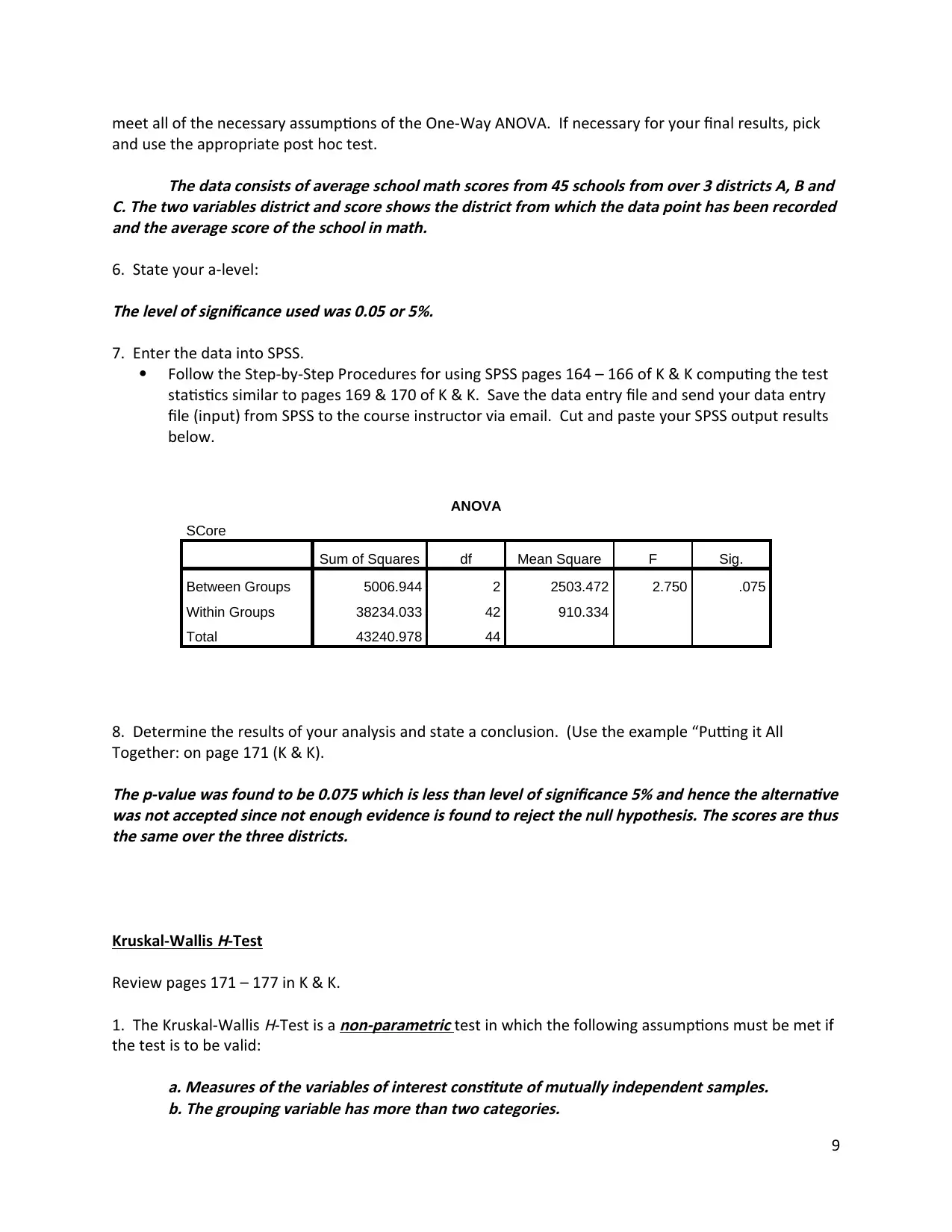
7. Enter the data into SPSS.
 Follow the Step-by-Step Procedures for using SPSS pages 164 – 166 of K & K computing the test
statistics similar to pages 169 & 170 of K & K. Save the data entry file and send your data entry
file (input) from SPSS to the course instructor via email. Cut and paste your SPSS output results
below.
ANOVA
SCore
Sum of Squares df Mean Square F Sig.
Between Groups 5006.944 2 2503.472 2.750 .075
Within Groups 38234.033 42 910.334
Total 43240.978 44
8. Determine the results of your analysis and state a conclusion. (Use the example “Putting it All
Together: on page 171 (K & K).
The p-value was found to be 0.075 which is less than level of significance 5% and hence the alternative
was not accepted since not enough evidence is found to reject the null hypothesis. The scores are thus
the same over the three districts.
Kruskal-Wallis
H-Test
Review pages 171 – 177 in K & K.
1. The Kruskal-Wallis
H-Test is a
non-parametric test in which the following assumptions must be met if
the test is to be valid:a. Measures of the variables of interest constitute of mutually independent samples.
b. The grouping variable has more than two categories.
9

c. The variables of interest are at least ordinal in scale of measurement.
2. Develop a (real or fictitious) research question that could be addressed by the Kruskal-Wallis
H-Test:To test whether the salary of different employee groups, namely minorities, men and women
are different in a company.
3. State the (real or fictitious) Null and Alternative Hypotheses:
H0: mean salary of women= mean salary of men= mean salary of minorities
Against
H1: At least one inequality among the salaries among the groups (alternate)
4. Make up a set of data to analyze in SPSS that would qualify for the use of the Kruskal-Wallis
H-Test.
Over-all have at least 10 – 15 data pints in each of the three groups for this exercise. Make sure that
data meet all of the necessary assumptions of the Kruskal-Wallis
H-Test. If necessary for your final
results, pick and use the appropriate post hoc test.
5. State you’re a-level:
The level of significance used was 0.05 or 5%.
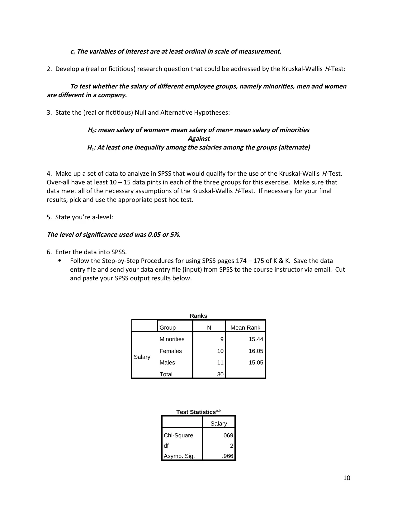
6. Enter the data into SPSS.
 Follow the Step-by-Step Procedures for using SPSS pages 174 – 175 of K & K. Save the data
entry file and send your data entry file (input) from SPSS to the course instructor via email. Cut
and paste your SPSS output results below.
Ranks
Group N Mean Rank
Salary
Minorities 9 15.44
Females 10 16.05
Males 11 15.05
Total 30
Test Statisticsa,b
Salary
Chi-Square .069
df 2
Asymp. Sig. .966
10

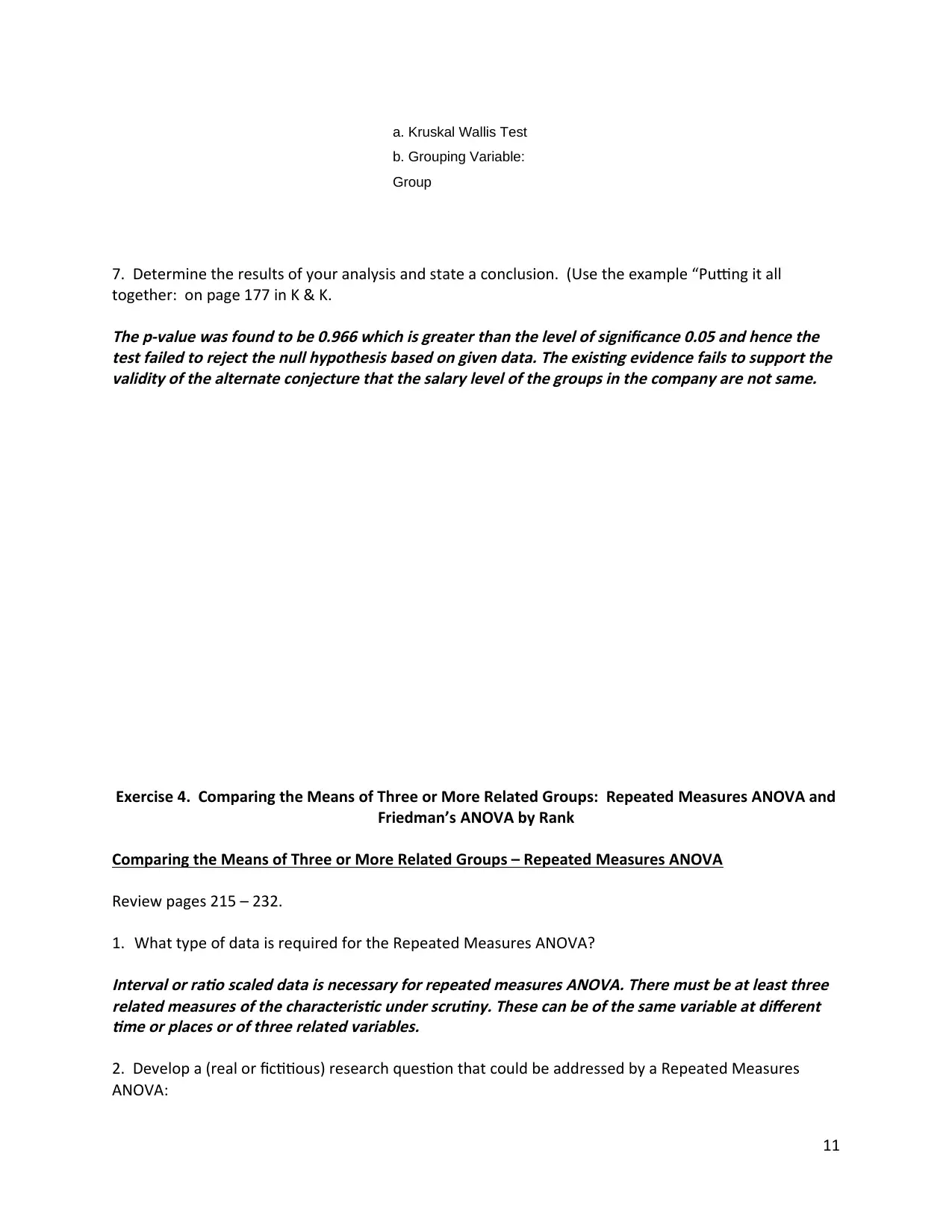
a. Kruskal Wallis Test
b. Grouping Variable:
Group
7. Determine the results of your analysis and state a conclusion. (Use the example “Putting it all
together: on page 177 in K & K.
The p-value was found to be 0.966 which is greater than the level of significance 0.05 and hence the
test failed to reject the null hypothesis based on given data. The existing evidence fails to support the
validity of the alternate conjecture that the salary level of the groups in the company are not same.
Exercise 4. Comparing the Means of Three or More Related Groups: Repeated Measures ANOVA and
Friedman’s ANOVA by Rank
Comparing the Means of Three or More Related Groups – Repeated Measures ANOVA
Review pages 215 – 232.
1. What type of data is required for the Repeated Measures ANOVA?
Interval or ratio scaled data is necessary for repeated measures ANOVA. There must be at least three
related measures of the characteristic under scrutiny. These can be of the same variable at different
time or places or of three related variables.
2. Develop a (real or fictitious) research question that could be addressed by a Repeated Measures
ANOVA:
11

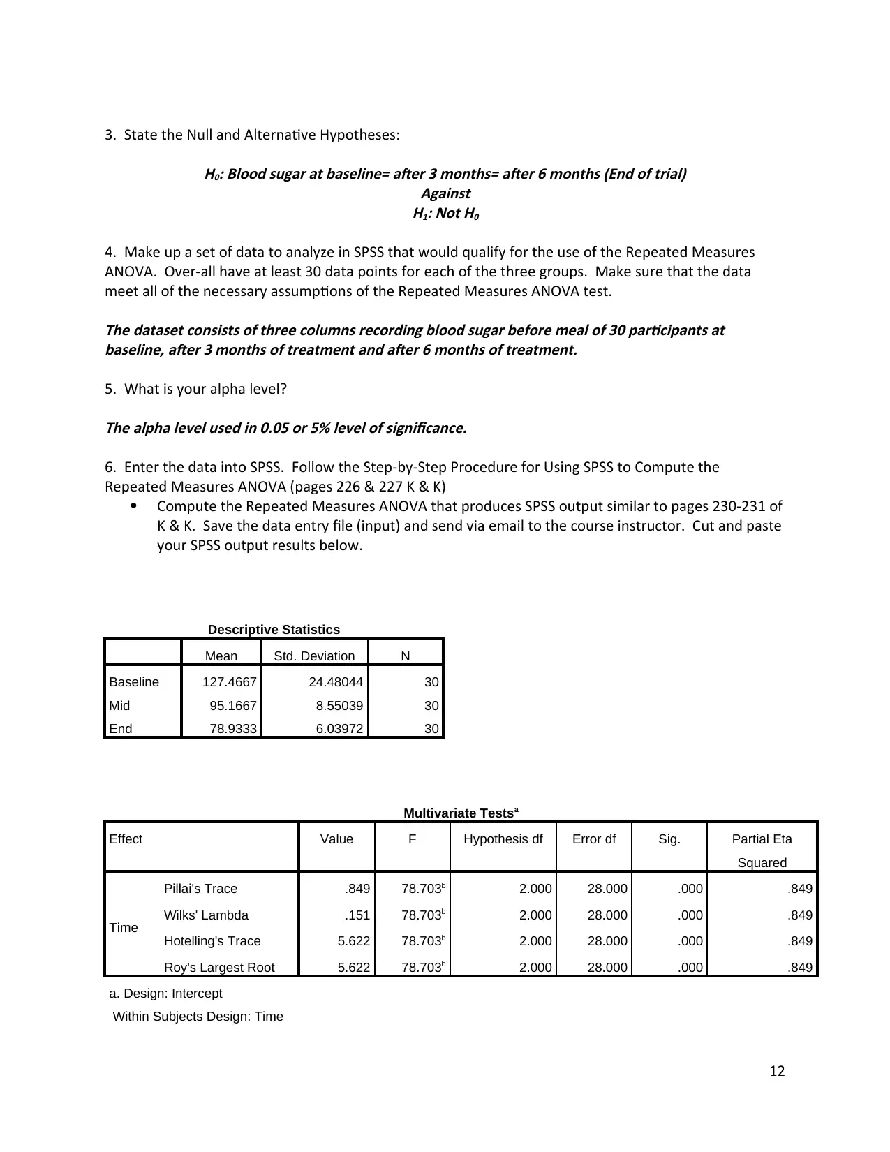
3. State the Null and Alternative Hypotheses:
H0: Blood sugar at baseline= after 3 months= after 6 months (End of trial)
Against
H1: Not H0
4. Make up a set of data to analyze in SPSS that would qualify for the use of the Repeated Measures
ANOVA. Over-all have at least 30 data points for each of the three groups. Make sure that the data
meet all of the necessary assumptions of the Repeated Measures ANOVA test.
The dataset consists of three columns recording blood sugar before meal of 30 participants at
baseline, after 3 months of treatment and after 6 months of treatment.
5. What is your alpha level?
The alpha level used in 0.05 or 5% level of significance.
6. Enter the data into SPSS. Follow the Step-by-Step Procedure for Using SPSS to Compute the
Repeated Measures ANOVA (pages 226 & 227 K & K)
 Compute the Repeated Measures ANOVA that produces SPSS output similar to pages 230-231 of
K & K. Save the data entry file (input) and send via email to the course instructor. Cut and paste
your SPSS output results below.
Descriptive Statistics
Mean Std. Deviation N
Baseline 127.4667 24.48044 30
Mid 95.1667 8.55039 30
End 78.9333 6.03972 30
Multivariate Testsa
Effect Value F Hypothesis df Error df Sig. Partial Eta
Squared
Time
Pillai's Trace .849 78.703b 2.000 28.000 .000 .849
Wilks' Lambda .151 78.703b 2.000 28.000 .000 .849
Hotelling's Trace 5.622 78.703b 2.000 28.000 .000 .849
Roy's Largest Root 5.622 78.703b 2.000 28.000 .000 .849
a. Design: Intercept
Within Subjects Design: Time
12