72160 Statistical Analysis Assignment 1, Semester 3, 2018 Report
VerifiedAdded on 2023/05/28
|17
|3444
|180
Report
AI Summary
This report presents a comprehensive statistical analysis assignment, structured into two main parts: planning research and exploratory analysis. Part A focuses on the research problem of social network impact on students, outlining target populations, explanatory and response variables, sampling methods, and data collection methods. Part B delves into exploratory analysis, including dataset descriptions, graphical and numerical explorations, and statistical enquiry processes. The analysis investigates the impact of alcohol consumption on life expectancy across different countries, employing graphical representations such as histograms and box plots, along with descriptive statistics and a one-way ANOVA model. The findings reveal insights into the relationship between alcohol consumption levels and average life expectancy, supported by statistical tests and descriptive summaries.
72160 Statistical Analysis Assignment 1, Semester 3, 2018
72 1 6 0 S TAT I S T I C A L A N A LY S E S
A S S I G N M E N T 1 R E P O R T
TRIMESTER 3, 2018
Prepared by <insert your LastNameFirstNameStudentID>
<insert the current Day Month Year>
pg. 1
72 1 6 0 S TAT I S T I C A L A N A LY S E S
A S S I G N M E N T 1 R E P O R T
TRIMESTER 3, 2018
Prepared by <insert your LastNameFirstNameStudentID>
<insert the current Day Month Year>
pg. 1
Paraphrase This Document
Need a fresh take? Get an instant paraphrase of this document with our AI Paraphraser
72160 Statistical Analysis Assignment 1, Semester 3, 2018
Table of Contents
Table of Contents
PART A. PLANNING RESEARCH 2
Introduction 2
1. Target Population 2
2. Explanatory and Response Variables 2
3. Sampling Method 3
4. Data Collection Method and Justification 3
PART B. EXPLORATORY ANALYSIS 4
Introduction 4
1. Statistical Enquiry Process 5
2. Dataset description 6
3. List of graphs and descriptive statistics for data exploration 6
4. Graphical Exploration 6
5. Numerical Exploration (Descriptive Statistics) 8
6. Summary of Results 8
7. Suggested Follow-up Investigations 9
C. APPENDICES (RAW SPSS OUTPUTS) 10
pg. 1
Table of Contents
Table of Contents
PART A. PLANNING RESEARCH 2
Introduction 2
1. Target Population 2
2. Explanatory and Response Variables 2
3. Sampling Method 3
4. Data Collection Method and Justification 3
PART B. EXPLORATORY ANALYSIS 4
Introduction 4
1. Statistical Enquiry Process 5
2. Dataset description 6
3. List of graphs and descriptive statistics for data exploration 6
4. Graphical Exploration 6
5. Numerical Exploration (Descriptive Statistics) 8
6. Summary of Results 8
7. Suggested Follow-up Investigations 9
C. APPENDICES (RAW SPSS OUTPUTS) 10
pg. 1
72160 Statistical Analysis Assignment 1, Semester 3, 2018
Part A. Planning Research
Introduction
The article has been constructed to address the following research problem.
"To address the negative consequences of social networks among high school students,
teachers are considering other after-school sports activities. Before going any further,
they want to gather information about how much time students spend now on optional
activities and how much time they spend on social networks."
The intermediate school was considered an important part of their day, so children have
the ability to play, have a chat, do homework, exercise, take music and other enrichment
classes and relax. In this article, the scholar has revised two topics related to school
activities. First, the characteristics of a child, a family, and work related to differences in
school activities of young people. Second, does participation in these events relate to
differences in child’s adaptation with regard to the later date in different activities, and
his/her time devoted to various activities including social media interaction. These issues
were addressed in a sample of 194 American children examined from fifth, sixth, and
seventh grade in a longitudinal study.
1. Target Population
The target population was selected from an intermediate school in the United States. The
school was selected randomly, but somehow on the basis of homogeneous financial
backgrounds of the families from which the students belong. The students from fifth,
sixth and seventh grades were selected in a stratified random sampling technique.
Guardians of the wards were also interviewed for their outlook on their children’s
extracurricular activities, and especially about their knowledge about the possible impact
of social media on their kids.
pg. 2
⊘ This is a preview!⊘
Do you want full access?
Subscribe today to unlock all pages.
Trusted by 1+ million students worldwide
72160 Statistical Analysis Assignment 1, Semester 3, 2018
2. Explanatory and Response Variables
Demographic details of the children were collected. Age, gender, and socioeconomic
status of the family were assessed to be three important explanatory factors. Total time
spent on social media websites, especially, any particular choice of timing for surfing
the internet was also considered as explanatory variables from the survey. The
financial condition of the family was also one of the explanatory variables in the study.
Other than social networking, students were evaluated for activities based on music,
outdoor and indoor games, and adventure sports activities. Interest levels of the students
for the activities were assessed from the performance and time taken to perform the
activities. The time spent on social media and on extracurricular activities was
considered as the dependent or outcome variable.
3. Sampling Method
The current study has expanded previous works and tested the use of time with the
children in fifth to seventh grade. The first objective was to identify the characteristics
of the child and the family in relation to children's activities after school. The second
goal was to investigate relationships within two years between social, emotional and
academic activities and rules for children. The longitudinal survey was conducted with
two types of sampling techniques. First, the schools were selected randomly from the
Texas province of the United States. Next, the students were selected from their
respective classes by using a stratified sampling method. The stratified sampling was
done considering the three classes as three strata.
4. Data Collection Method and Justification
The scholar sent letters describing the study to the parents of fifth, sixth and seventh
class students from nine transition schools. The study was formalized in an
environmental perspective, and parents spoke of a more recent experience to adapt to
methodologies taught in school. They were asked to return the form with information
about basic demographic and children's information about their family. The researchers
chose schools because they had a high proportion of children who were Americans and
whites. In addition, students were available after school, either in schools or in adjoining
pg. 3
Paraphrase This Document
Need a fresh take? Get an instant paraphrase of this document with our AI Paraphraser
72160 Statistical Analysis Assignment 1, Semester 3, 2018
areas. 50% of the family (n = 96) returned the forms. Of those who agreed to provide
information about their child, 78 percent agreed to participate. The demographic profile
of the volunteer children in each school was established with respect to the parental race,
gender and education. From the ready-to-do interview pool, all American families (n =
78) are selected as participants. The scholar chose white and non-Hispanic children from
the groups of available participants, using a stratified random sampling plan that
provided roughly the same number of girls and boys.
There was no difference between the children selected for education and those who were
not selected in terms of gender, lunch scholarships or school transfer. 48% were
American. 52% were girls. 55% lived in the same family home. The parents also
provided the weekly schedule of their kids, and the total time invested in extracurricular
activities was cross verified from the students.
The sampling methodology and data collection procedures can be justified based on the
structure of the research. The strata of schools were chosen to explore and establish the
results based on the difference between American and other children. Also, frequent
access to social media for the majority of the students was also an essential component
of research. It is to be noted that scholar also wanted some students from non-American
communities, who have the less financially affluent background and access to social
media sites. Also, random sampling was essential to avoid any possible bias due to the
homogeneity of the sample subjects. The type of extracurricular activities was also an
important aspect in data collection method. The scholar wanted specifically to collect the
data on time invested in the sports and sports-related activities.
Part B. Exploratory Analysis
Introduction
The alcohol-related mortality rate is estimated in several populations, but few studies
have yielded reliable results in mortality and age and gender-related to alcohol. The
death register contains information on the main and associated causes of death and
provides an individual assessment of the proportion of alcohol consumption in mortality.
The data for life expectancy with alcohol consumption has been used to investigate the
pg. 4
72160 Statistical Analysis Assignment 1, Semester 3, 2018
effect of alcohol, and to assess the influence of over-consumption of alcohol on the
population of the sample countries in the sample data. The data set summarizes
information from 45 countries about the average life expectancy of citizens. The study
examined the question of whether the average life expectancy of citizens at three levels
(low, medium, high) or alcohol consumption per adult citizen per year was different.
The present article researches on the impact of alcohol consumption on the average life
expectancy in several countries. Interest was also revealed for the descriptive summary
of consumptions of all the counties. Also, a one-way ANOVA model was constructed to
find the difference between life expectancies for three levels of alcohol consumption. A
post-hoc analysis for pair-wise comparison was also done to find the significant
difference in life expectancy for the alcohol consumption levels.
1. Statistical Enquiry Process
The sample data was scrutinized for the type of the variables. The variable indicating
level of alcohol consumption was converted from a string level variable to a numerical
variable by introducing a categorical variable with three values. High level of
consumption was denoted by “3” and the low level was assigned “1”. The ordinality
nature of the categorical variable was preserved. The researcher tried to assess the
difference in average life expectancy for three different levels of alcohol consumptions.
The research question was framed as whether excess alcohol consumption adversely
impacts the average life expectancy of the people across different counties in the world.
A set of hypotheses were constructed for inferential analysis of the research objective.
The null hypothesis was constructed as follows,
H0: Alcohol consumption level had no impact on the average life expectancy of people
( μ1=μ2=μ3 )
The alternate two-tailed hypothesis to be tested at a 5% level of significance was
constructed as follows,
pg. 5
⊘ This is a preview!⊘
Do you want full access?
Subscribe today to unlock all pages.
Trusted by 1+ million students worldwide
72160 Statistical Analysis Assignment 1, Semester 3, 2018
HA: Alcohol consumption level had a statistically significant effect on the average life
expectancy of people ( μ1≠μ2≠μ3 ) . Hence, there exists at least one group of countries
with different alcohol consumption than the other two groups.
2. Dataset description
According to the data received, 33.33% percent (N = 45) of all alcohol-related cases
were for all three reported levels of consumption. Probable deaths caused alcohol
consumption was responsible for the loss of life expectancy of people from 45 countries
across the globe. In the low alcohol consumption category the average life expectancy
was 82.53 years (SD = 6.81). The average life expectancy at average consumption level
was 70.45 years (SD = 9.05), and for high consumption group, the average life
expectancy was 63.27 Years (SD = 5.74). Normality of the life expectancy was checked
by Shapiro-Wilk test. At 5% level of significance the variable was found to be
significantly normally distributed (W = 0.965, p = 0.195). The choice of the dependent
variable as average life expectancy was evident. The control or independent variable was
the categorical alcohol consumptions. No missing values were observed, and the
descriptive summary revealed that the mean of average life expectancies was 73.76
years (SD = 10.77). Median of the distribution was 73 years. Hence, 50% of the
countries had an average life expectancy less than 73 years. The 95% confidence
interval for the mean life expectancy of the total data set was evaluated for the
population mean as 70.52 years to 76.99 years.
3. List of graphs and descriptive statistics for data exploration
The normality of the life expectancy was explored by histogram fitted normal curve.
A side-by-side box plot was constructed to visually represent the difference in central
tendency of life expectancy and the spread for three levels of alcohol consumptions.
Mean and standard deviations were calculated to descriptively summarize the life
expectancy of the sample.
Shapiro-Wilk test statistic was used to check the normality of the average life
expectancy.
pg. 6
Paraphrase This Document
Need a fresh take? Get an instant paraphrase of this document with our AI Paraphraser
72160 Statistical Analysis Assignment 1, Semester 3, 2018
A one-way ANOVA with F-statistics was used to assess the difference in life
expectancies for three consumption levels.
4. Graphical Exploration
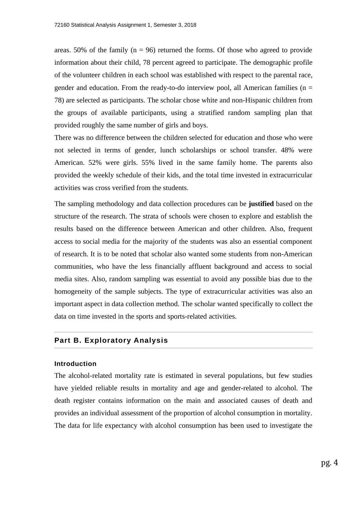
Figure 1 below reflected that the life expectancy data for 45 countries was normally
distributed with mean = 73.76 years (SD = 10.77).
Figure 1: Histogram of Life Expectancy of the 45 Countries
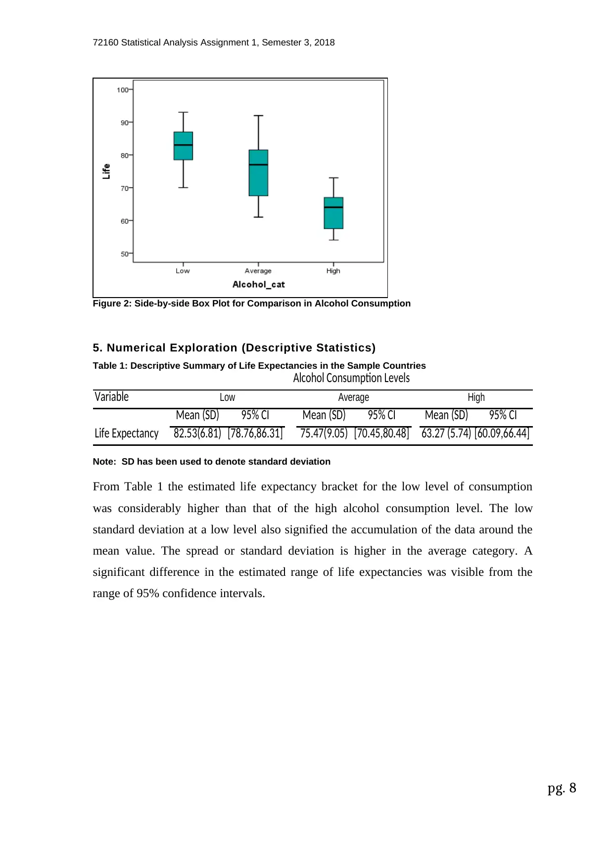
Figure 2 provides a clear display of the central location of the life expectancies for three
categories of alcohol consumptions. It was noted that average life expectancy (LE) was
normally distributed and the median LE across the globe was way higher for low alcohol
consumption. The spread or the middle 50% observations was greater for average
consumption level. A positive skewness can also be identified from the box plot of
average category. For a high level of alcohol consumption, the median LE was near to
65 years of age with a high positive skewness. Hence, differences in life expectancies
were found to depend on the consumption level of alcohols.
pg. 7
A one-way ANOVA with F-statistics was used to assess the difference in life
expectancies for three consumption levels.
4. Graphical Exploration
Figure 1 below reflected that the life expectancy data for 45 countries was normally
distributed with mean = 73.76 years (SD = 10.77).
Figure 1: Histogram of Life Expectancy of the 45 Countries
Figure 2 provides a clear display of the central location of the life expectancies for three
categories of alcohol consumptions. It was noted that average life expectancy (LE) was
normally distributed and the median LE across the globe was way higher for low alcohol
consumption. The spread or the middle 50% observations was greater for average
consumption level. A positive skewness can also be identified from the box plot of
average category. For a high level of alcohol consumption, the median LE was near to
65 years of age with a high positive skewness. Hence, differences in life expectancies
were found to depend on the consumption level of alcohols.
pg. 7
72160 Statistical Analysis Assignment 1, Semester 3, 2018
Figure 2: Side-by-side Box Plot for Comparison in Alcohol Consumption
5. Numerical Exploration (Descriptive Statistics)
Table 1: Descriptive Summary of Life Expectancies in the Sample Countries
Variable
Mean (SD) 95% CI Mean (SD) 95% CI Mean (SD) 95% CI
Life Expectancy 82.53(6.81) [78.76,86.31] 75.47(9.05) [70.45,80.48] 63.27 (5.74) [60.09,66.44]
Low Average High
Alcohol Consumption Levels
Note: SD has been used to denote standard deviation
From Table 1 the estimated life expectancy bracket for the low level of consumption
was considerably higher than that of the high alcohol consumption level. The low
standard deviation at a low level also signified the accumulation of the data around the
mean value. The spread or standard deviation is higher in the average category. A
significant difference in the estimated range of life expectancies was visible from the
range of 95% confidence intervals.
pg. 8
⊘ This is a preview!⊘
Do you want full access?
Subscribe today to unlock all pages.
Trusted by 1+ million students worldwide
72160 Statistical Analysis Assignment 1, Semester 3, 2018
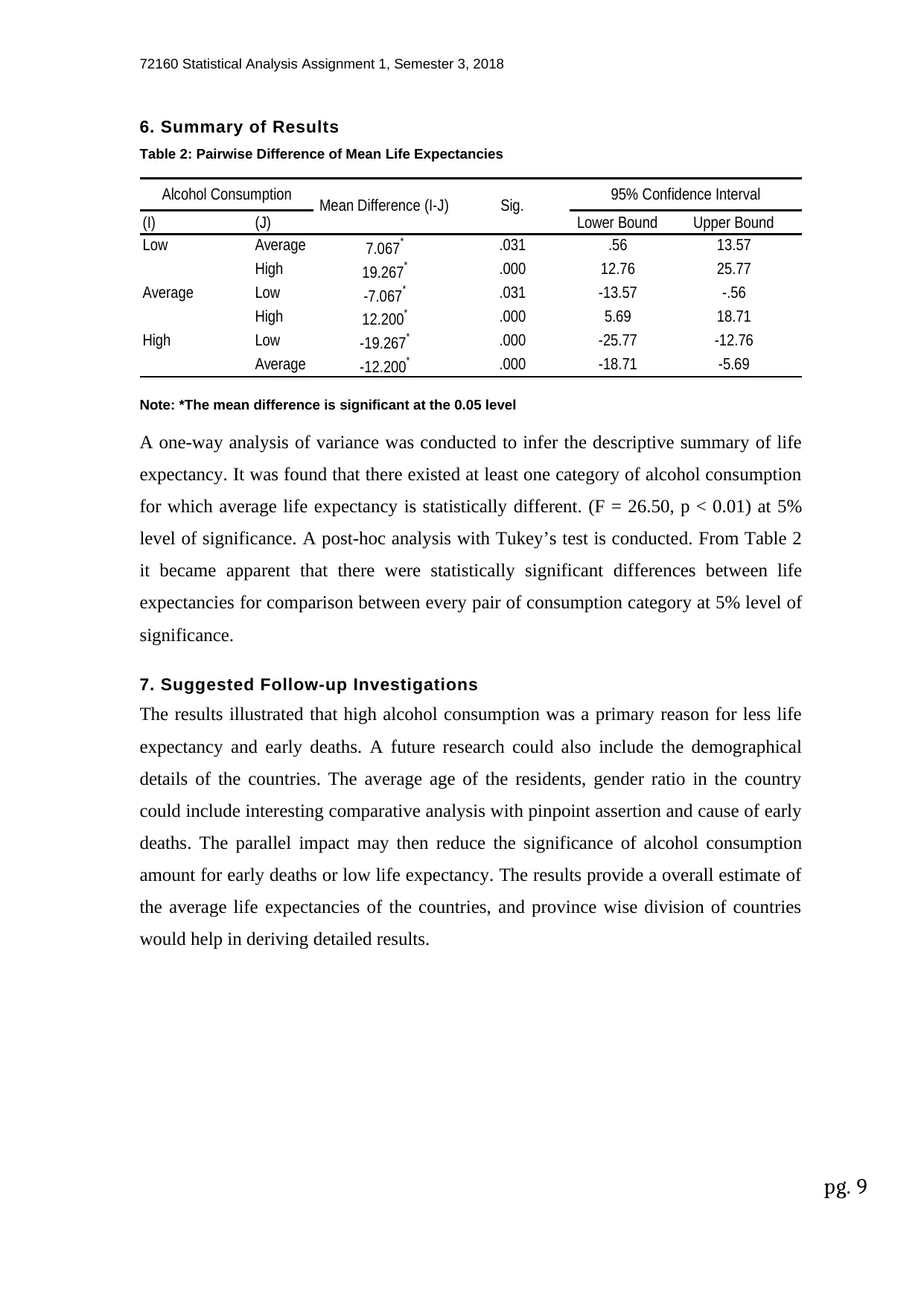
6. Summary of Results
Table 2: Pairwise Difference of Mean Life Expectancies
(I) (J) Lower Bound Upper Bound
Low Average 7.067* .031 .56 13.57
High 19.267* .000 12.76 25.77
Average Low -7.067* .031 -13.57 -.56
High 12.200* .000 5.69 18.71
High Low -19.267* .000 -25.77 -12.76
Average -12.200* .000 -18.71 -5.69
95% Confidence IntervalAlcohol Consumption Mean Difference (I-J) Sig.
Note: *The mean difference is significant at the 0.05 level
A one-way analysis of variance was conducted to infer the descriptive summary of life
expectancy. It was found that there existed at least one category of alcohol consumption
for which average life expectancy is statistically different. (F = 26.50, p < 0.01) at 5%
level of significance. A post-hoc analysis with Tukey’s test is conducted. From Table 2
it became apparent that there were statistically significant differences between life
expectancies for comparison between every pair of consumption category at 5% level of
significance.
7. Suggested Follow-up Investigations
The results illustrated that high alcohol consumption was a primary reason for less life
expectancy and early deaths. A future research could also include the demographical
details of the countries. The average age of the residents, gender ratio in the country
could include interesting comparative analysis with pinpoint assertion and cause of early
deaths. The parallel impact may then reduce the significance of alcohol consumption
amount for early deaths or low life expectancy. The results provide a overall estimate of
the average life expectancies of the countries, and province wise division of countries
would help in deriving detailed results.
pg. 9
Paraphrase This Document
Need a fresh take? Get an instant paraphrase of this document with our AI Paraphraser
72160 Statistical Analysis Assignment 1, Semester 3, 2018
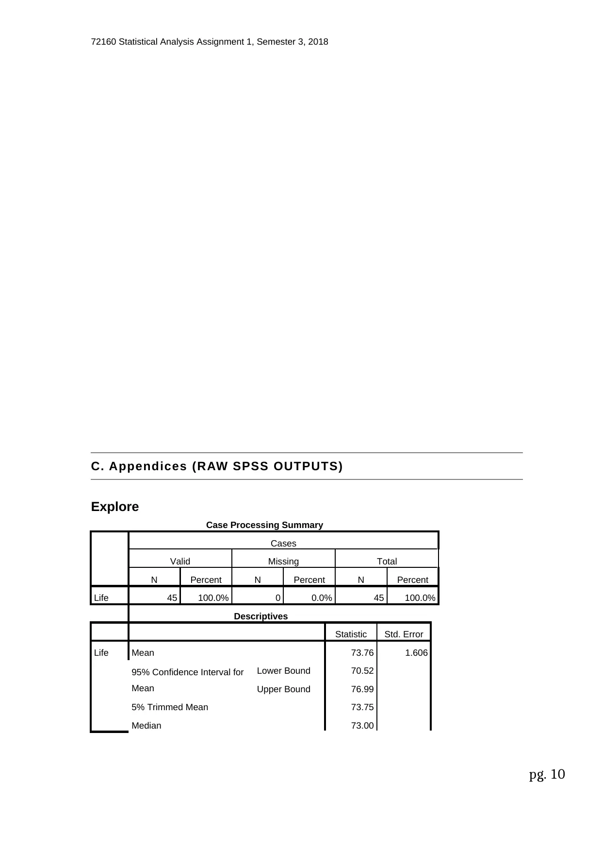
C. Appendices (RAW SPSS OUTPUTS)
Explore
Case Processing Summary
Cases
Valid Missing Total
N Percent N Percent N Percent
Life 45 100.0% 0 0.0% 45 100.0%
Descriptives
Statistic Std. Error
Life Mean 73.76 1.606
95% Confidence Interval for
Mean
Lower Bound 70.52
Upper Bound 76.99
5% Trimmed Mean 73.75
Median 73.00
pg. 10
72160 Statistical Analysis Assignment 1, Semester 3, 2018
Variance 116.098
Std. Deviation 10.775
Minimum 54
Maximum 93
Range 39
Interquartile Range 18
Skewness .008 .354
Kurtosis -1.036 .695
Tests of Normality
Kolmogorov-Smirnova Shapiro-Wilk
Statistic df Sig. Statistic df Sig.
Life .093 45 .200* .965 45 .195
*. This is a lower bound of the true significance.
a. Lilliefors Significance Correction
Life
pg. 11
⊘ This is a preview!⊘
Do you want full access?
Subscribe today to unlock all pages.
Trusted by 1+ million students worldwide
1 out of 17
Related Documents


Your All-in-One AI-Powered Toolkit for Academic Success.
+13062052269
info@desklib.com
Available 24*7 on WhatsApp / Email
![[object Object]](/_next/static/media/star-bottom.7253800d.svg)
Unlock your academic potential
Copyright © 2020–2026 A2Z Services. All Rights Reserved. Developed and managed by ZUCOL.