Statistical Analysis for Decision Making: STAT1060 Assignment 2
VerifiedAdded on 2022/11/11
|10
|1087
|152
Homework Assignment
AI Summary
This assignment solution for STAT1060, focusing on statistical analysis for decision-making, addresses four key questions. Question 1 explores convenience sampling, data types (discrete), and appropriate graphical representations (bar charts) to analyze card counts. Question 2 delves into continuous and categorical variables, using histograms and column charts to compare asset liability ratios for closed and operational businesses, incorporating descriptive statistics and hypothesis testing with t-tests. Question 3 involves hypothesis testing to compare packaging abilities using t-tests. Question 4 analyzes a contingency table and calculates probabilities, employing chi-square tests to determine the relationship between income and lookup variables, providing a comprehensive statistical analysis with Excel output and interpretations.
STATISTICS
STAT1060
STUDENT ID:
[Pick the date]
STAT1060
STUDENT ID:
[Pick the date]
Paraphrase This Document
Need a fresh take? Get an instant paraphrase of this document with our AI Paraphraser
Question 1
a) Convenience sampling is the underlying sampling technique that has been used for the given
variable. This is reflected from the fact that responses with regards to number of cards have
been obtained from respondents that are available. The researcher has not ensured that the
sample is representative of the population owing to which bias would be present.
b) As cards count has to be a integral value, thereby the underlying variable is discrete in nature.
Further, it is not a categorical variable and hence nominal and ordinal scales would not apply.
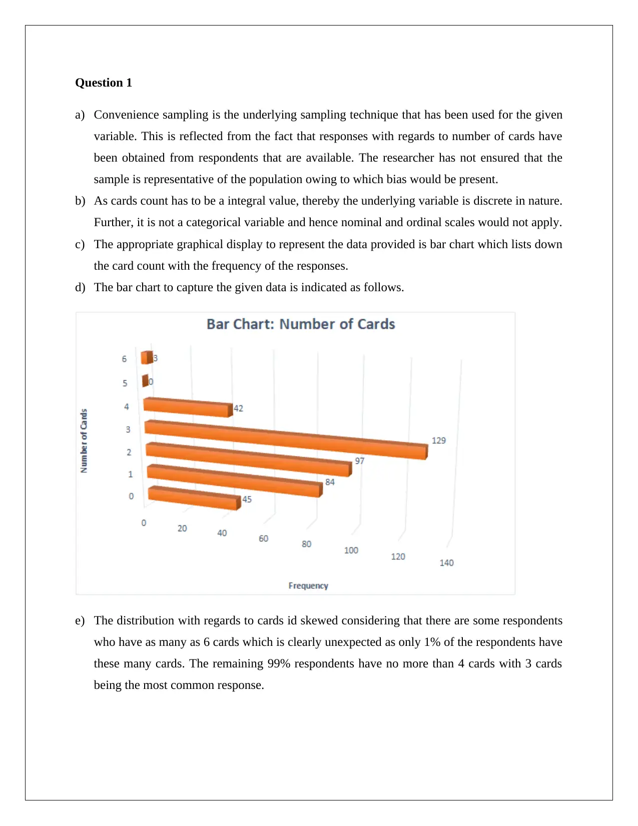
c) The appropriate graphical display to represent the data provided is bar chart which lists down
the card count with the frequency of the responses.
d) The bar chart to capture the given data is indicated as follows.
e) The distribution with regards to cards id skewed considering that there are some respondents
who have as many as 6 cards which is clearly unexpected as only 1% of the respondents have
these many cards. The remaining 99% respondents have no more than 4 cards with 3 cards
being the most common response.
Question 2
a) The asset liability ratio variable is expressed in numerical terms and also the values are both
integers as well as decimals. As a result, the given variable would be continuous in nature.
With regards to operational variable, the possible choices are a yes or no which implies that
the variable is categorical and suitable type is nominal as there is no natural order to
arrangement possible for the responses.
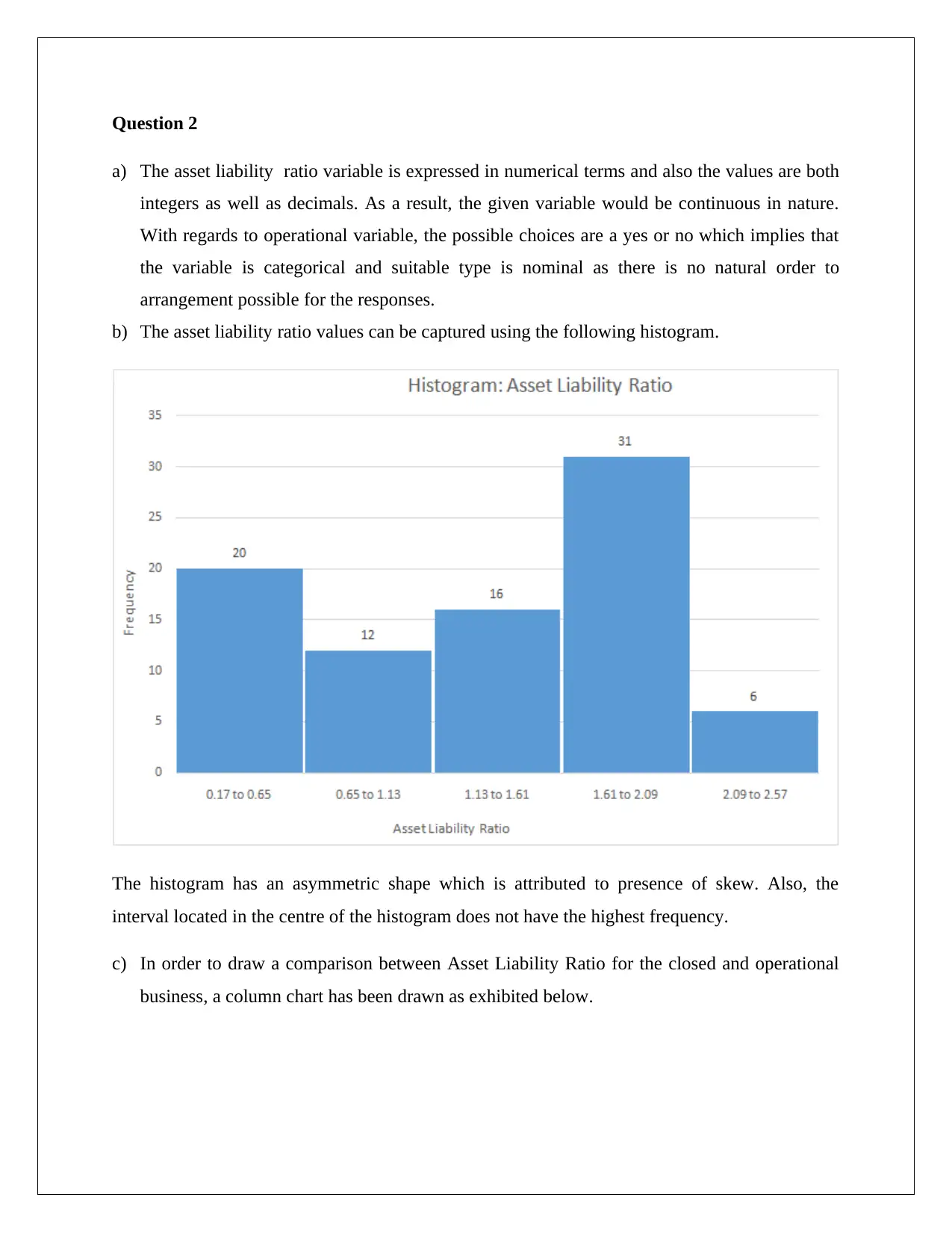
b) The asset liability ratio values can be captured using the following histogram.
The histogram has an asymmetric shape which is attributed to presence of skew. Also, the
interval located in the centre of the histogram does not have the highest frequency.
c) In order to draw a comparison between Asset Liability Ratio for the closed and operational
business, a column chart has been drawn as exhibited below.
⊘ This is a preview!⊘
Do you want full access?
Subscribe today to unlock all pages.

Trusted by 1+ million students worldwide
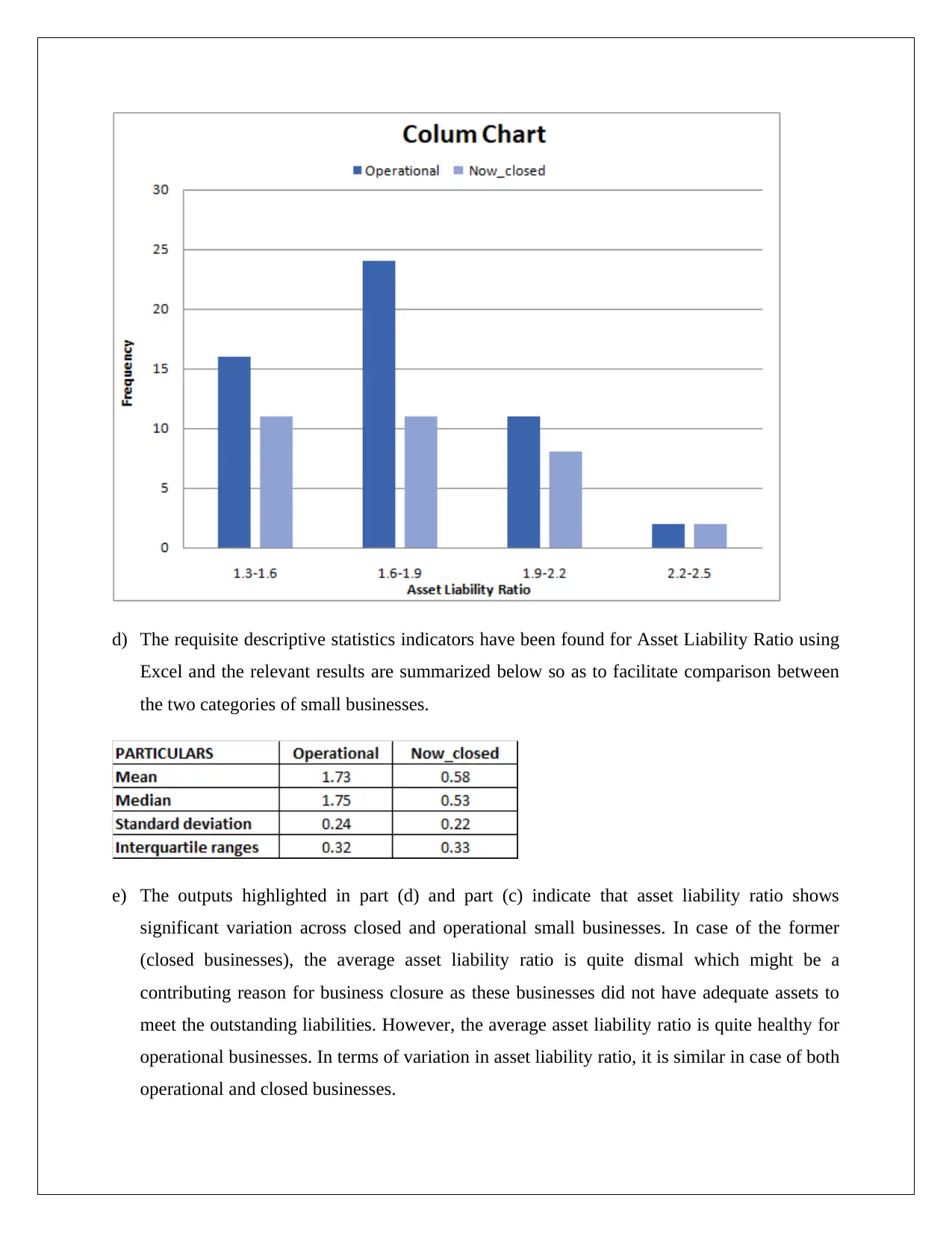
d) The requisite descriptive statistics indicators have been found for Asset Liability Ratio using
Excel and the relevant results are summarized below so as to facilitate comparison between
the two categories of small businesses.
e) The outputs highlighted in part (d) and part (c) indicate that asset liability ratio shows
significant variation across closed and operational small businesses. In case of the former
(closed businesses), the average asset liability ratio is quite dismal which might be a
contributing reason for business closure as these businesses did not have adequate assets to
meet the outstanding liabilities. However, the average asset liability ratio is quite healthy for
operational businesses. In terms of variation in asset liability ratio, it is similar in case of both
operational and closed businesses.
Paraphrase This Document
Need a fresh take? Get an instant paraphrase of this document with our AI Paraphraser
f) 1) Mean asset liability ratio (Operational small businesses) = 1.73
Standard deviation for asset liability ratio (Operational small businesses) = 0.24
Mean + 1 standard deviation = 1.73+0.24 = 1.97
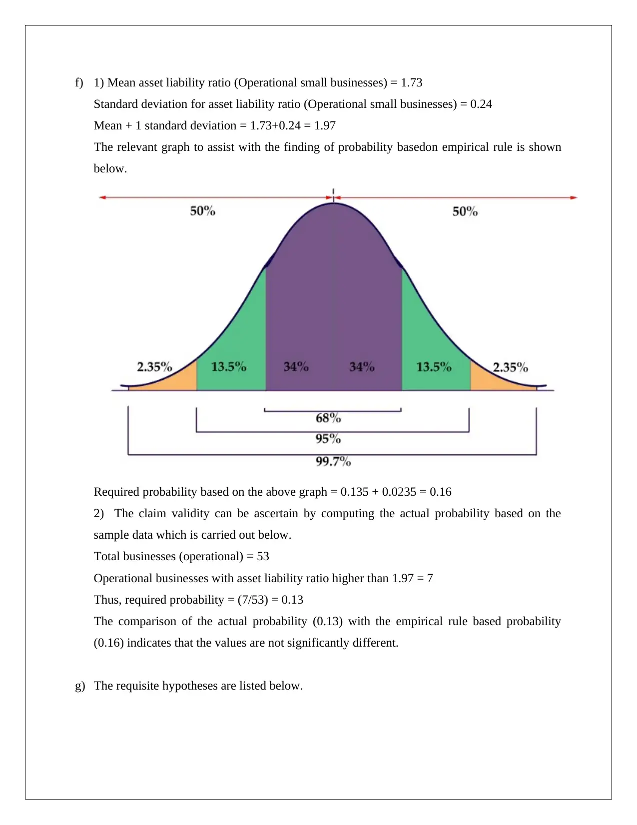
The relevant graph to assist with the finding of probability basedon empirical rule is shown
below.
Required probability based on the above graph = 0.135 + 0.0235 = 0.16
2) The claim validity can be ascertain by computing the actual probability based on the
sample data which is carried out below.
Total businesses (operational) = 53
Operational businesses with asset liability ratio higher than 1.97 = 7
Thus, required probability = (7/53) = 0.13
The comparison of the actual probability (0.13) with the empirical rule based probability
(0.16) indicates that the values are not significantly different.
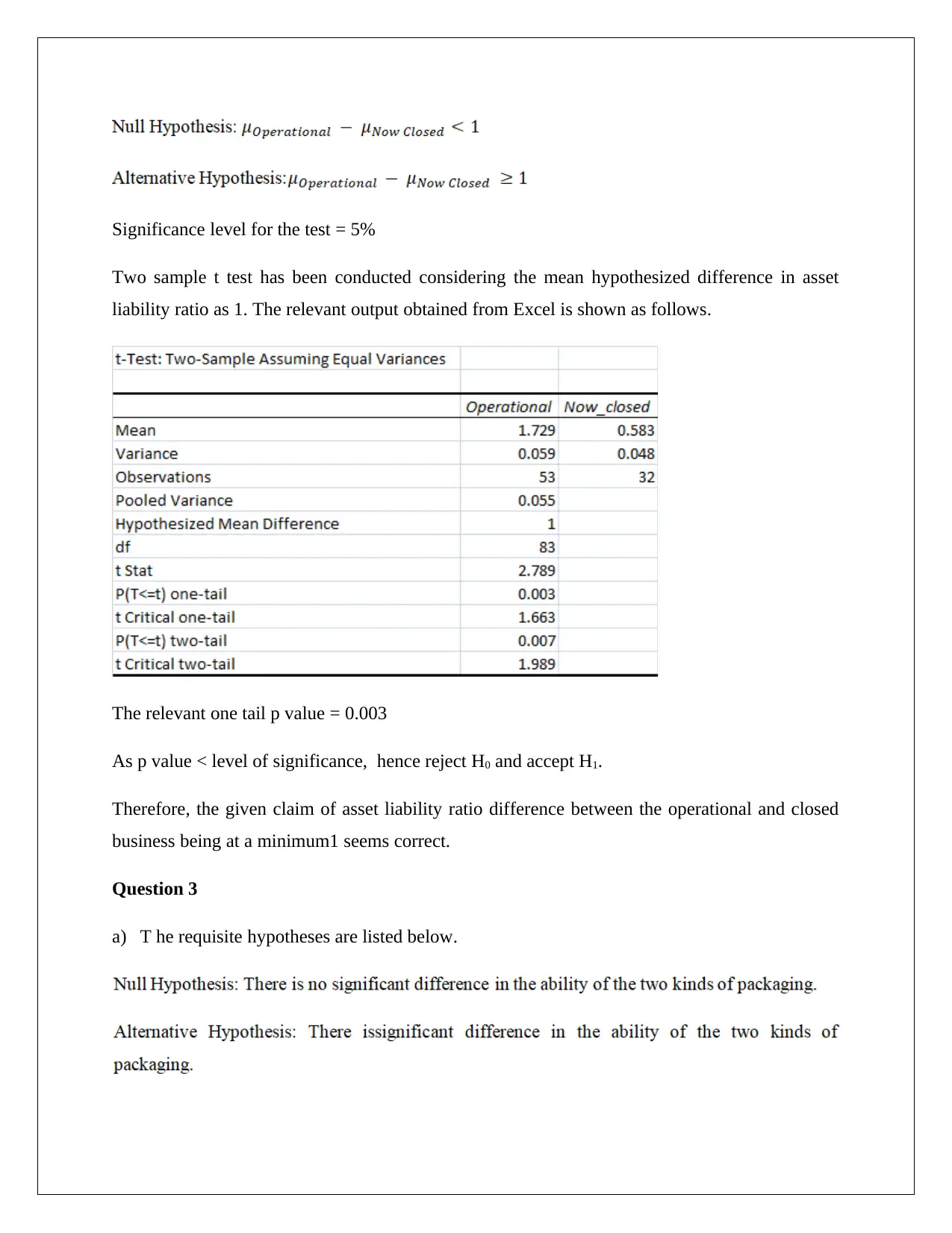
g) The requisite hypotheses are listed below.
Significance level for the test = 5%
Two sample t test has been conducted considering the mean hypothesized difference in asset
liability ratio as 1. The relevant output obtained from Excel is shown as follows.
The relevant one tail p value = 0.003
As p value < level of significance, hence reject H0 and accept H1.
Therefore, the given claim of asset liability ratio difference between the operational and closed
business being at a minimum1 seems correct.
Question 3
a) T he requisite hypotheses are listed below.
⊘ This is a preview!⊘
Do you want full access?
Subscribe today to unlock all pages.

Trusted by 1+ million students worldwide
Significance level for the test = 5%
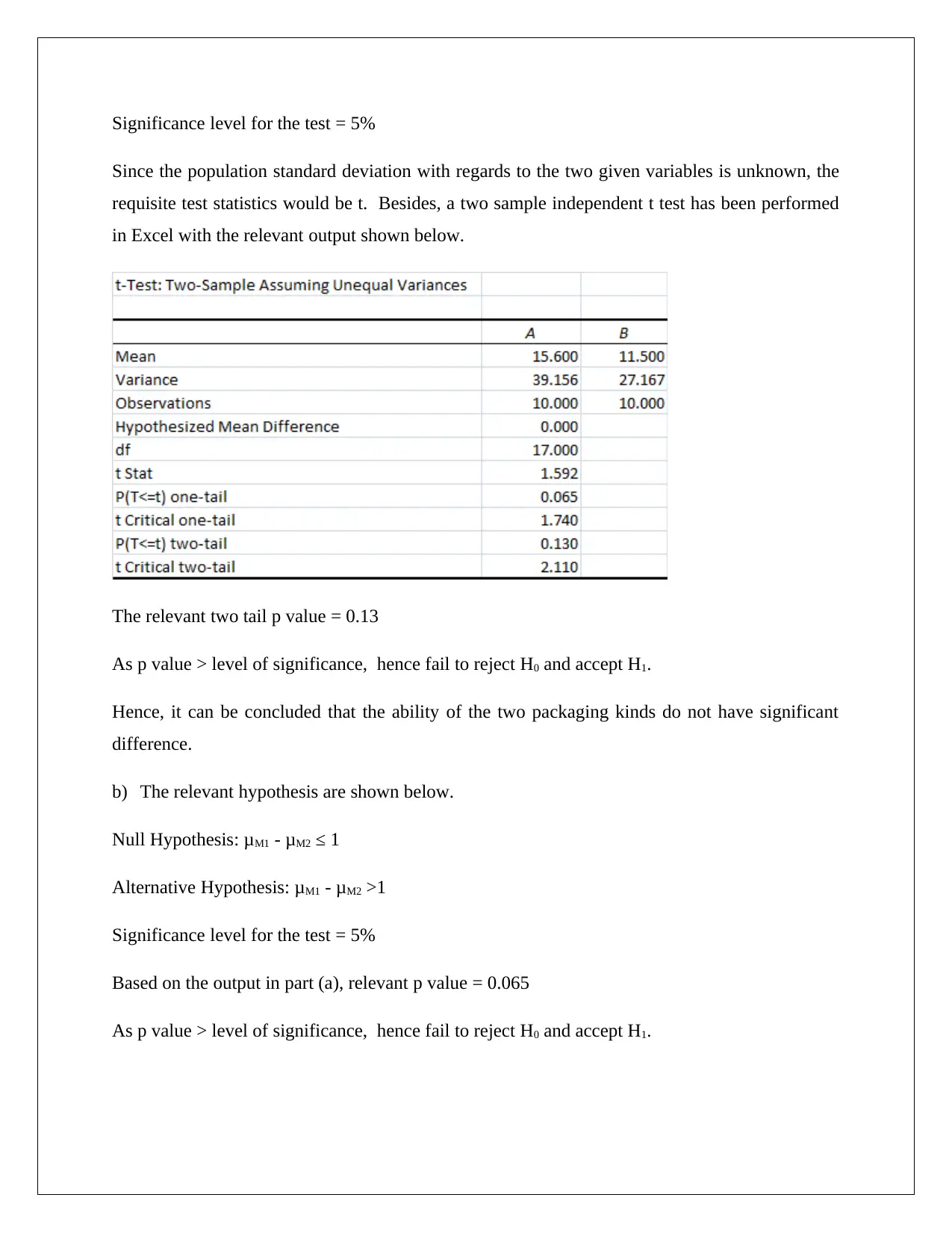
Since the population standard deviation with regards to the two given variables is unknown, the
requisite test statistics would be t. Besides, a two sample independent t test has been performed
in Excel with the relevant output shown below.
The relevant two tail p value = 0.13
As p value > level of significance, hence fail to reject H0 and accept H1.
Hence, it can be concluded that the ability of the two packaging kinds do not have significant
difference.
b) The relevant hypothesis are shown below.
Null Hypothesis: μM1 - μM2 ≤ 1
Alternative Hypothesis: μM1 - μM2 >1
Significance level for the test = 5%
Based on the output in part (a), relevant p value = 0.065
As p value > level of significance, hence fail to reject H0 and accept H1.
Paraphrase This Document
Need a fresh take? Get an instant paraphrase of this document with our AI Paraphraser
Hence, the claim made by the employee from manufacturing department is supported by the
given data.
Question 4
The contingency table is summarized
(a) The requisite probability is computed as follows.
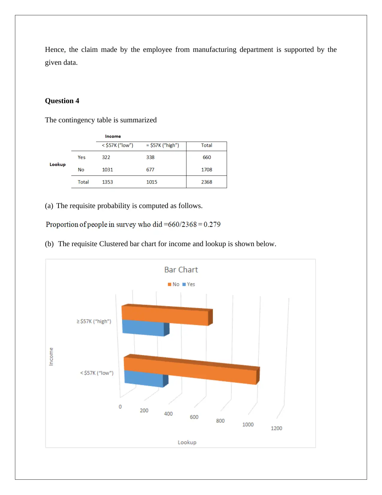
(b) The requisite Clustered bar chart for income and lookup is shown below.
given data.
Question 4
The contingency table is summarized
(a) The requisite probability is computed as follows.
(b) The requisite Clustered bar chart for income and lookup is shown below.
The above bar chart indicates that the people included in the survey who responded yes for both
low and high income level are few in number. However, the people included in the survey who
responded no for both low and high income level are quite high.
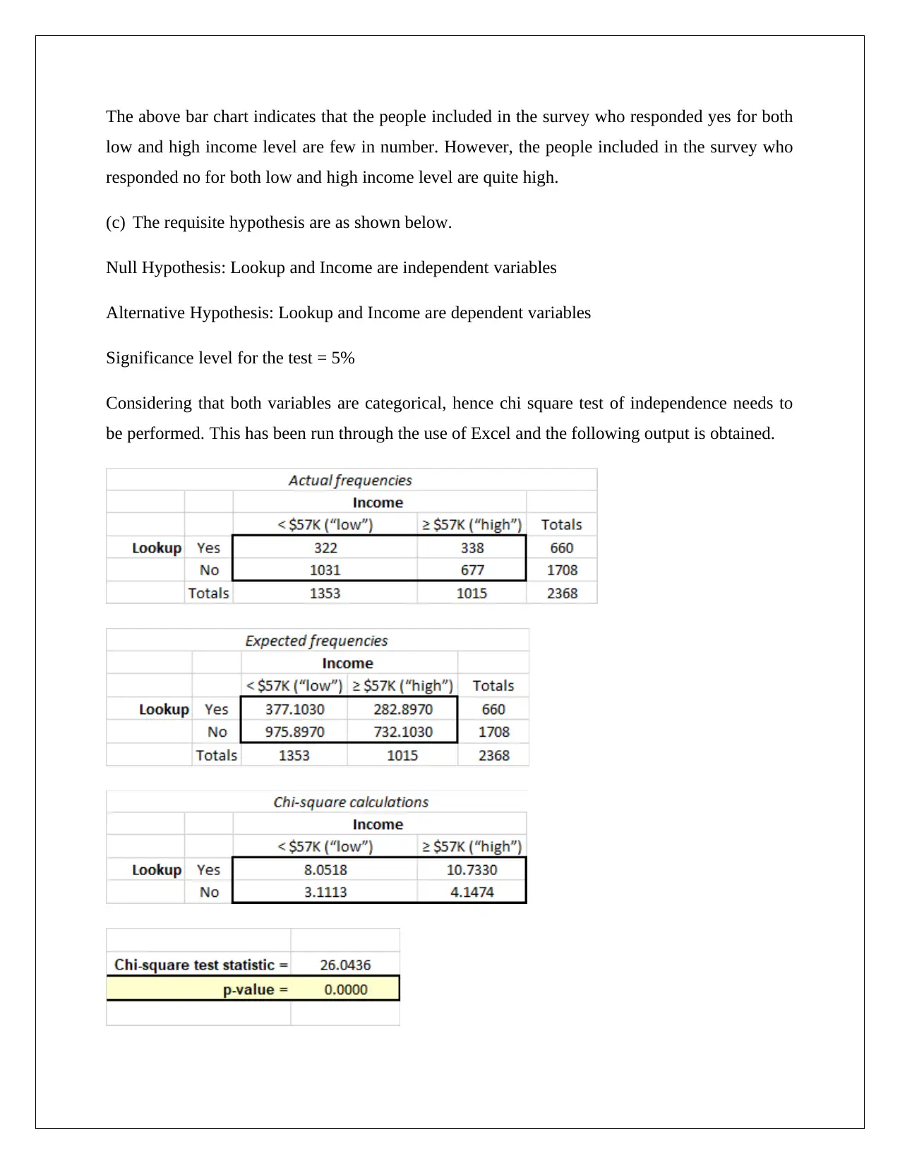
(c) The requisite hypothesis are as shown below.
Null Hypothesis: Lookup and Income are independent variables
Alternative Hypothesis: Lookup and Income are dependent variables
Significance level for the test = 5%
Considering that both variables are categorical, hence chi square test of independence needs to
be performed. This has been run through the use of Excel and the following output is obtained.
⊘ This is a preview!⊘
Do you want full access?
Subscribe today to unlock all pages.

Trusted by 1+ million students worldwide
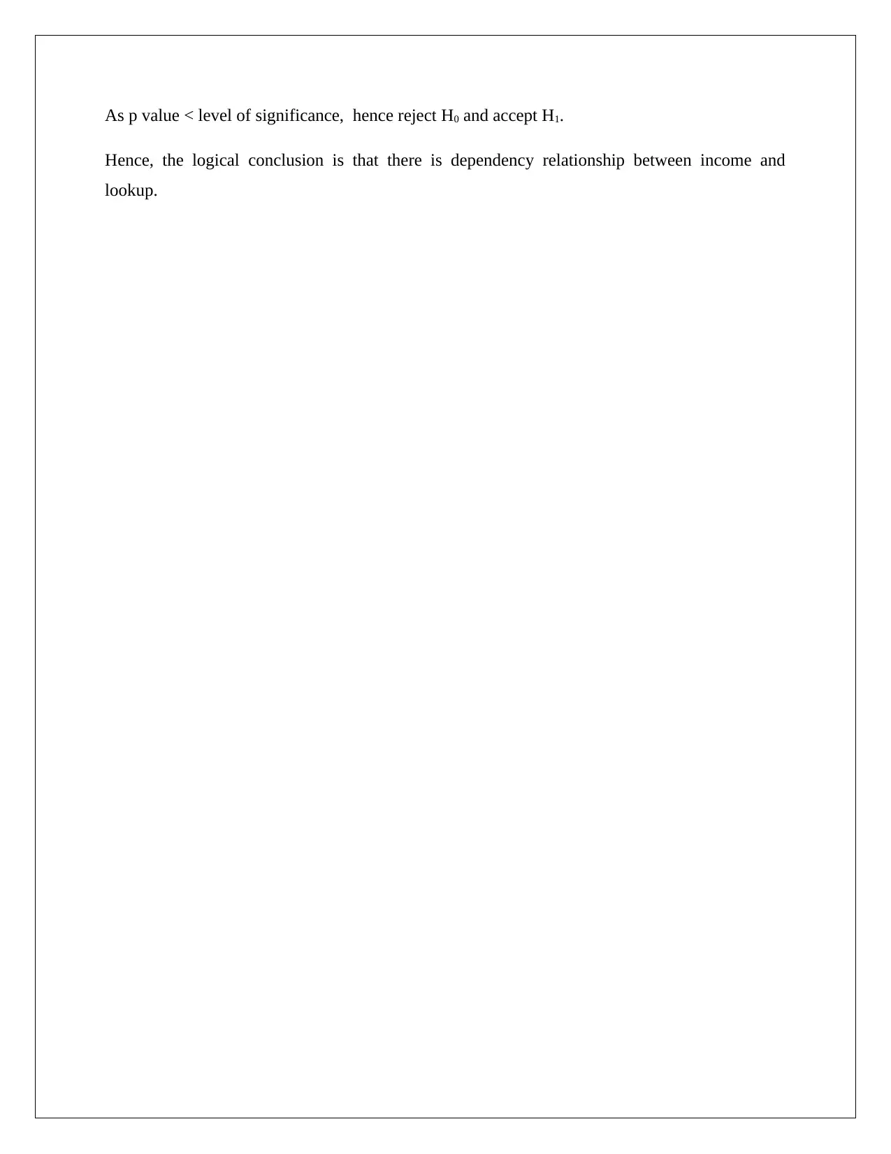
As p value < level of significance, hence reject H0 and accept H1.
Hence, the logical conclusion is that there is dependency relationship between income and
lookup.
Hence, the logical conclusion is that there is dependency relationship between income and
lookup.
1 out of 10
Related Documents
Your All-in-One AI-Powered Toolkit for Academic Success.
+13062052269
info@desklib.com
Available 24*7 on WhatsApp / Email
![[object Object]](/_next/static/media/star-bottom.7253800d.svg)
Unlock your academic potential
Copyright © 2020–2026 A2Z Services. All Rights Reserved. Developed and managed by ZUCOL.


