HI6007: Statistics, Research Methods, and Business Decision Making

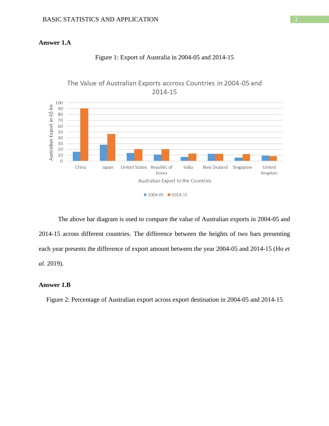
This assignment demonstrates the application of statistical techniques to solve business problems. It begins with data visualization using bar diagrams and discusses the Australian export data, comparing export values and proportions across different countries over two years. The assignment then analyzes umbrella sales data, constructing frequency tables, histograms, and ogives to understand the distribution of sales. Descriptive statistics, including mean, median, mode, standard deviation, and correlation, are calculated for retail turnover per capita and final consumption expenditure. The assignment also includes regression analysis to examine the relationship between these two variables, interpreting the regression equation, coefficients, and goodness-of-fit measures. The analysis provides insights into the relationship between retail turnover and final consumption expenditure, concluding with a summary of the findings and the statistical methods used.

Running head: BASIC STATISTICS AND APPLICATION
Basic Statistics and Application
Name of the Student:
Name of the University:
Author’s Note:

1BASIC STATISTICS AND APPLICATION
Table of Contents
Introduction:....................................................................................................................................2
Answer 1.A......................................................................................................................................3
Answer 1.B......................................................................................................................................3
Answer 1.C......................................................................................................................................4
Answer 2.A & B..............................................................................................................................5
Answer 2.C......................................................................................................................................5
Answer 2.D......................................................................................................................................6
Answer 2.E......................................................................................................................................7
Answer 2.F.......................................................................................................................................7
Answer 3.A......................................................................................................................................7
Answer 3.B......................................................................................................................................8
Answer 3.C......................................................................................................................................9
Answer 3.D....................................................................................................................................10
Answer 3.E....................................................................................................................................10
Answer 3.F.....................................................................................................................................11
Answer 3.G....................................................................................................................................11
Answer 3.H....................................................................................................................................12
Reference.......................................................................................................................................13

2BASIC STATISTICS AND APPLICATION
Introduction:
Statistical techniques have a major role in case of solving critical problems on the basis
of different types of data. Mainly there are two types of data: Qualitative and Quantitative. Again
quantitative data is of two types: Continuous and Discrete. Binomial, nominal and ordinal data
are three types of qualitative data. These all types of data follow a certain distribution like
normal distribution and binomial distribution, depending upon their nature and number of
observations. Now, specific statistical techniques are there to work efficiently and unbiasedly on
these distributions and data for proper analysis in solving business problems and decision
making. Few examples are discussed below:
Production managers use random sampling techniques to modify or regulate the rank of
materials in terms of quality. Random sampling is also used by the accountants at the time of
audit and by the policy makers of a company to investigate the employee’s efficiency.
Correlation is used by the financial department to correlate the business associated
variables and regression is used to judge the relation among those variables.
Forecasting is used in supply chain management and to predict the revenue and sales of a
profit making institution.
This type of practices is very general in business practices. There is some complicated
analysis which is practiced by the business professionals via computer packages or soft wares
that performs statistical analysis. In the below section some basic problems are solved and
discussed by using statistical techniques on the given data. In the end, a conclusion part
summarizes the findings.

3BASIC STATISTICS AND APPLICATION
Answer 1.A
Figure 1: Export of Australia in 2004-05 and 2014-15
The above bar diagram is used to compare the value of Australian exports in 2004-05 and
2014-15 across different countries. The difference between the heights of two bars presenting
each year presents the difference of export amount between the year 2004-05 and 2014-15 (Ho et
al. 2019).
Answer 1.B
Figure 2: Percentage of Australian export across export destination in 2004-05 and 2014-15

4BASIC STATISTICS AND APPLICATION
The above diagram shows the percentage of exports of Australia to different countries in
year 2004-05 and 2014-15.
Answer 1.C
The figure 1 presents the value of export of 2004-05 and 2014-15, broken down by
country of export destination. Figure 1 shows that the export amount has increased in 2014-15
for all the countries except UK and New Zealand. The figure 2 presents the percentage of export
to the export destination for both the years 2004-05 and 2014-15. The figure 2 shows that
Australia is exporting a large proportion of total export to China than before and less goods to
rest of the countries. Combining both the figures, it can be concluded that the export amount of
Australia has increased to each countries but the proportion of export is different from the
previous year. More specifically, Australian export is concentrating towards China.

5BASIC STATISTICS AND APPLICATION
Answer 2.A & B
Range Frequency Relative
Frequency
Cumulative
Frequency
Relative
Cumulative
Frequency
31-40 2 0.05 2 0.05
41-50 4 0.1 6 0.15
51-60 8 0.2 14 0.35
61-70 11 0.275 25 0.625
71-80 8 0.2 33 0.825
81-90 5 0.125 38 0.95
91-100 2 0.05 40 1
Table 1: Frequency table of umbrella sales
The above tables shows the frequency, relative frequency, cumulative frequency and
relative cumulative frequency for each class. Frequency is number of occurrence of an outcome.
Relative frequency is the ration of frequency of an outcome and the total number of outcomes
(Leptokaropoulos and Staszek 2019). Relative cumulative frequency is the sum of the relative
frequency for the outcomes less than or equal to the given outcome.
Answer 2.C
Figure 3: Histogram of the relative frequency

6BASIC STATISTICS AND APPLICATION
The figure 3 presents the histogram of relative frequency. The histogram shows that the
sales of umbrella is normally distributed as the shape of the diagram matches to the bell shaped
normal curve (Saghir, Akber Abbasi and Faraz 2019).
Answer 2.D
Figure 4: Ogive for the sales of umbrella

7BASIC STATISTICS AND APPLICATION
An ogive is a cumulative frequency graph. The above figure is obtained from the given
data of sales of umbrella (Suhane 2018).
Answer 2.E
Form the table 1, it is obtained that the proportion of grades less than 60 is 0.35.
Answer 2.F
Form the table 1, it is obtained that the proportion of grades more than 70 is (1-0.625) =
0.375.
Answer 3.A
Figure 5: Line diagram with a secondary axis to present two variables against time.

8BASIC STATISTICS AND APPLICATION
To describe the descriptive measure the average value is taken for retail turnover per
capita and final consumption expenditure and to present the time series data for both the
variables in a single diagram, a secondary axis is added. On the vertical axis average retail
turnover per capita and average final consumption expenditure is presented and on the horizontal
axis presents the year. Now, there are two lines in the chart presenting two variables over the
year (Brockett 2015).
Answer 3.B
Figure 6: Scatter diagram presenting relationship between two variables

9BASIC STATISTICS AND APPLICATION
The above scatter diagram presenting the relationship between retail turnover per capita
and final consumption expenditure where the dependent variables is retail turnover per capita
and the final consumption expenditure is independent variable. The dependent variable is always
plotted on the vertical axis and the independent variable on the horizontal axis in order to
interpret the result properly (Güçlü et al. 2015).
Answer 3.C
Statistical Measures Retail Turnover Per
Capita
Final Consumption
Expenditure
Mean 2205.76 146019.85
Median 2180.20 139137.00
Mode 2852.80
Standard Deviation 543.19 46904.33
Variance 295059.60 2200016261.88
Coefficient of Variation 0.25 0.32
Range 1558.70 151259.00
Minimum 1455.90 81889.00
Maximum 3014.60 233148.00
1st Quartile 1652.95 103558.50

10BASIC STATISTICS AND APPLICATION
3rd Quartile 2793.40 192800.50
Table 2: Descriptive statistics for the two variables.
The summary statistics of the retail turnover per capita and final consumption
expenditure is presented in the above table. The average value of retail turnover per capita and
final consumption expenditure are 2205.76 and 146019.85 respectively. The spread of retail
turnover per capita and final consumption expenditure are 543.19 and 46904.23 respectively
(Daniel and Cross 2018).
Answer 3.D
Variables Retail Turnover Per
Capita
Final Consumption
Expenditure
Retail Turnover Per Capita 1
Final Consumption
Expenditure 0.988 1
Table 3: Coefficient of correlation table
The table shows the coefficient correlation between final consumption expenditure and
retail turnover per capita which is equal to 0.988. The value is too close to 1. Therefore, the
relation is strong between the two variables (Gruber and Vigfusson 2018).
Answer 3.E
Regression Statistics
Multiple R 0.988
R Square 0.976
Adjusted R Square 0.975
Standard Error 85.273
Observations 131
Table 4.a: Summary output of regression
Coefficients Standard Error t Stat P-value
Intercept 535.53 24.45 21.91 0.00
Final Consumption 0.01 0.00 71.74 0.00

11BASIC STATISTICS AND APPLICATION
Expenditure
Table 4.b: Regression result
The estimated linear regression equation is mentioned below:
Y =535.53+(0.01∗X )
Where, Y= Retail turnover per capita and X= Final consumption expenditure. The
coefficient of intercept term is 535.53 which is significant at 1% level of significance which
implies that the initial value of Y (when X=0) is 535.53. The coefficient of X is 0.01 which is
statistically significant at 1% significance level. This implies one unit change in X will change
the Y by 0.01 unit (King and Giles 2018).
Answer 3.F
The table 4.a shows the summary of the regression which contains the values of multiple
R, R square and adjusted R square. The value of R2 is 0.976 that implies that the final
consumption expenditure can predict 97.6% of the retail turnover per capita (Berger, Maurer and
Celli 2018).
Answer 3.G
From the table 4.b the t-test can be explained for the slope coefficient. The null
hypothesis of the test is H0: β equals to 0 and the alternative hypothesis is HA: β not equals to 0.
The p-value is for the H0 against the HA. The p-value is 0.000 which is enough evidence to reject
the null hypothesis and accept the alternative hypothesis that the coefficient is not equal to zero
(McManus 2015). The positive value of t-stat implies that the p-value for the negative slope co-
efficient is 0.00. That means the slope coefficient is positive and statistically significant.