Statistical Analysis and Data Interpretation Homework Assignment

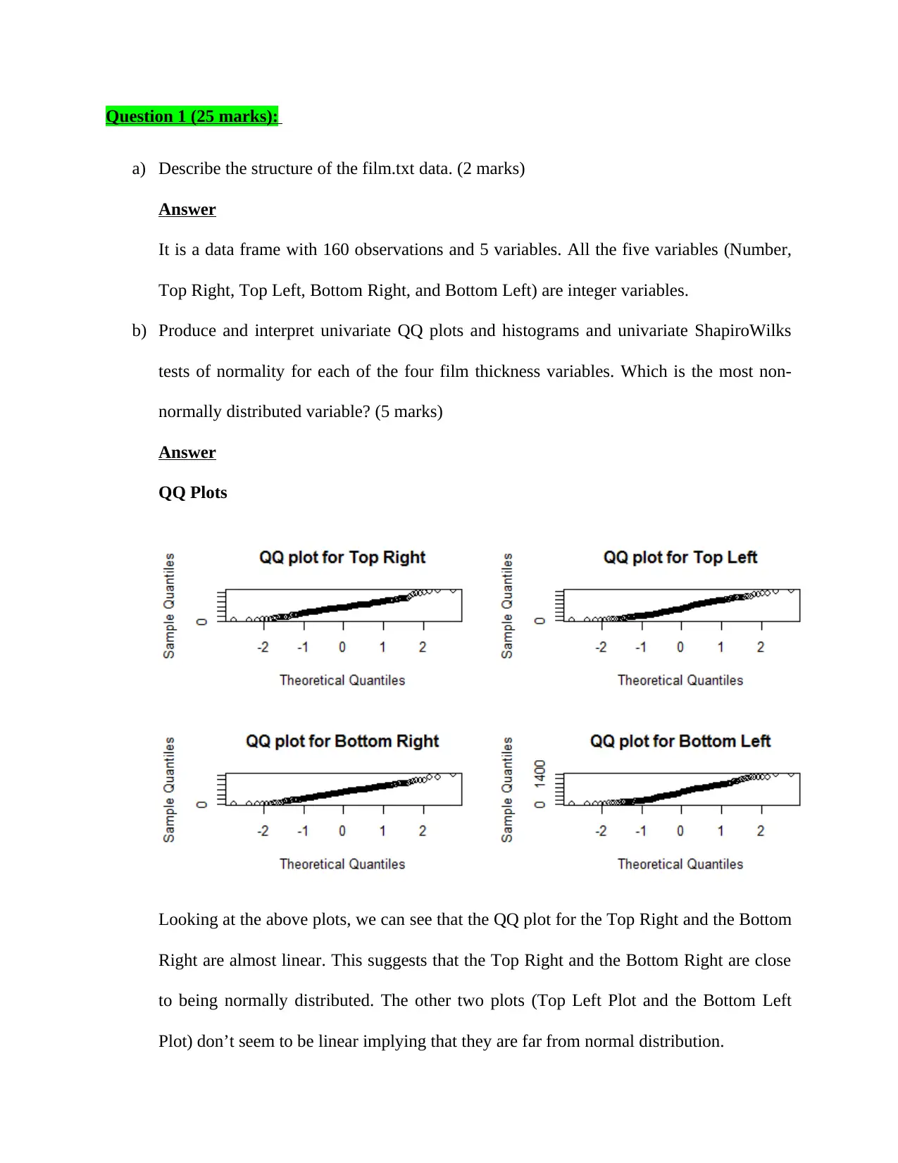
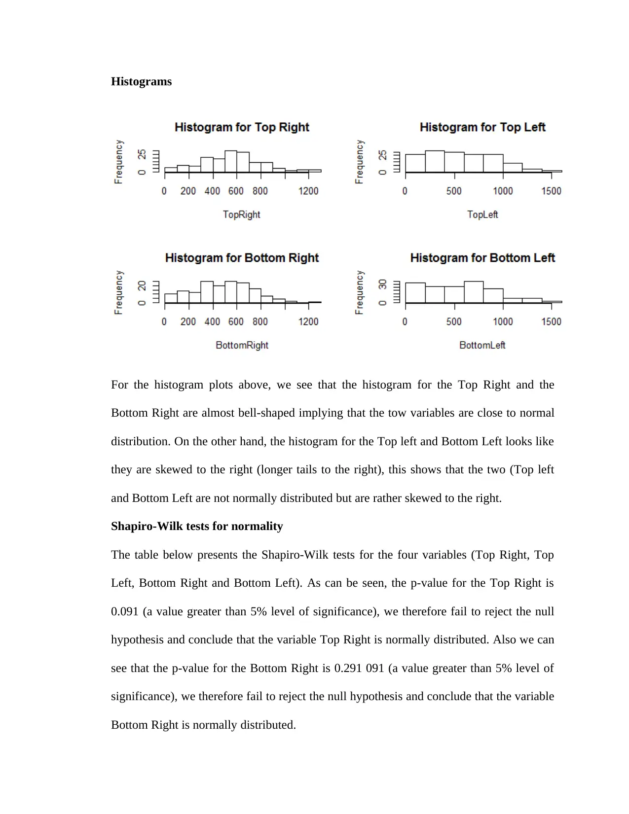
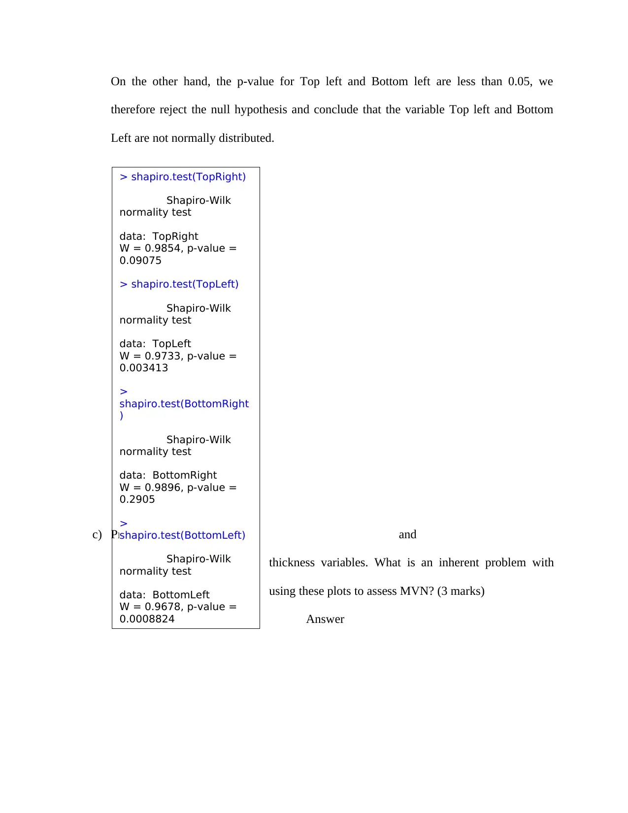
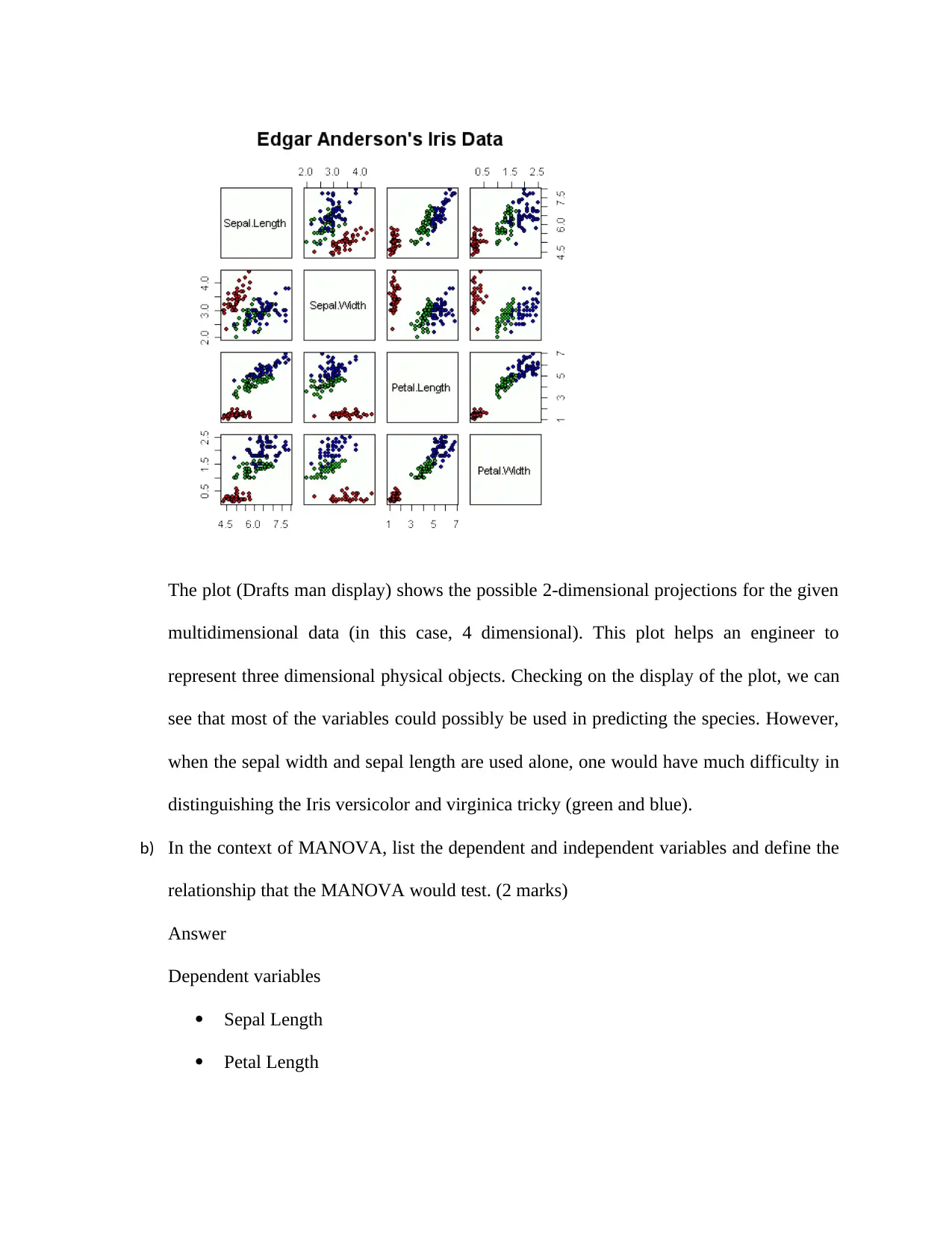
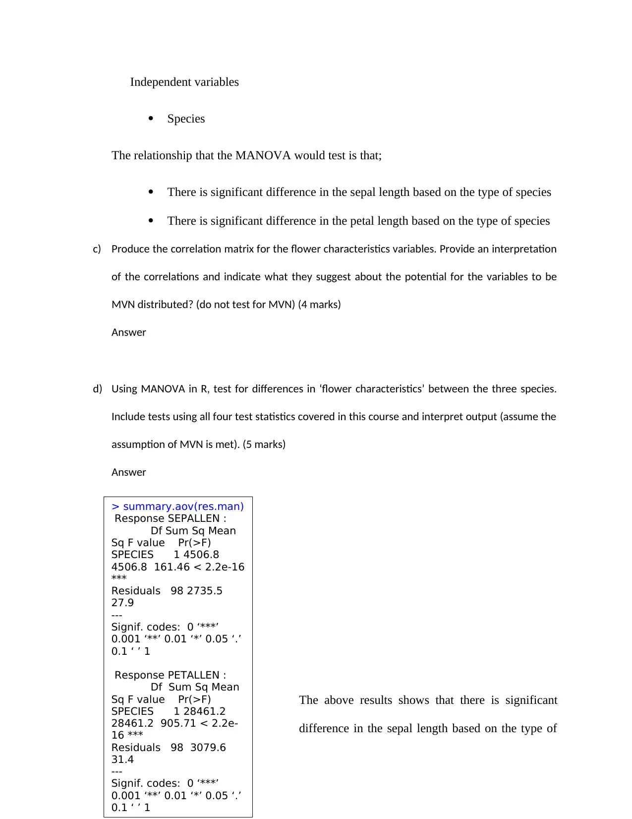
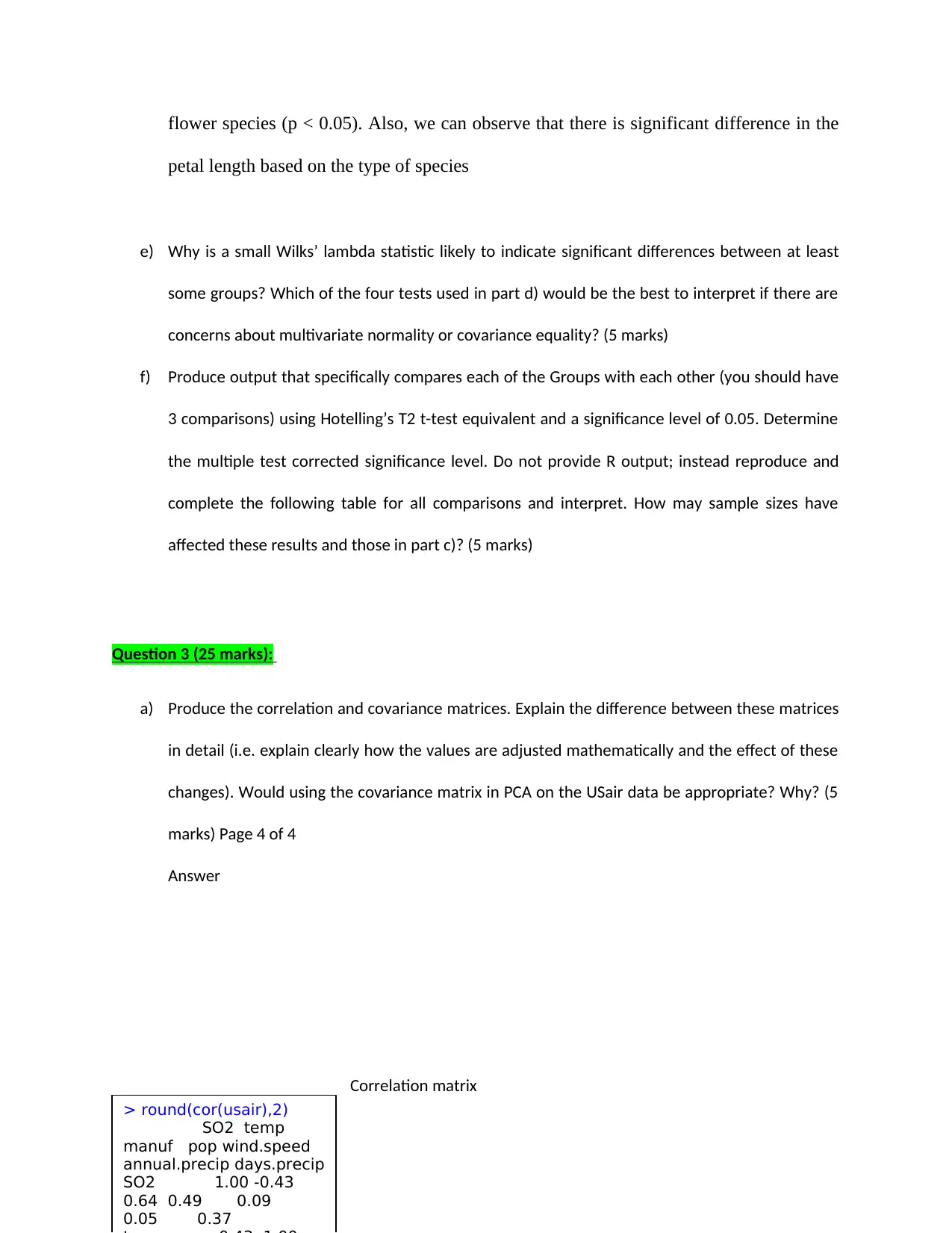
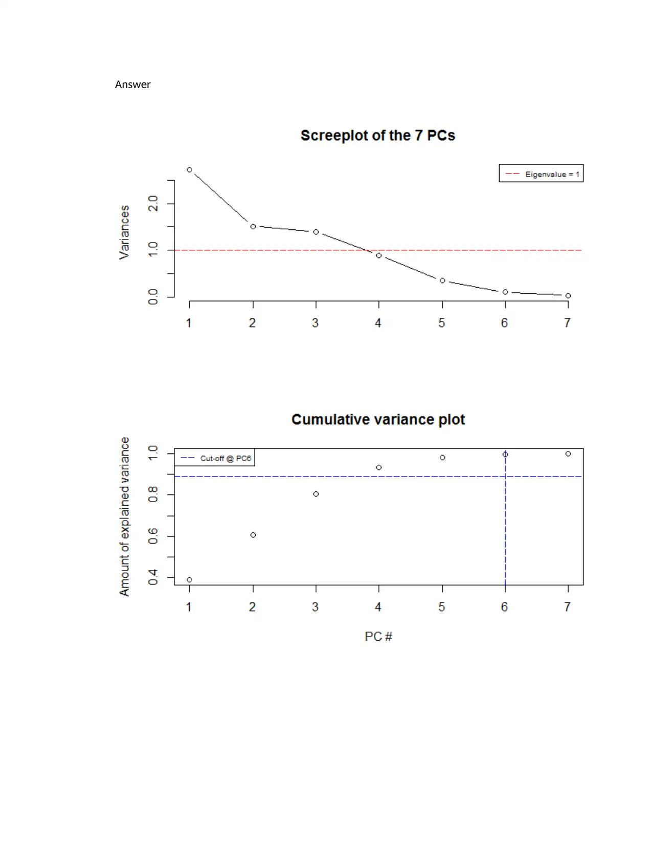
This homework assignment provides a comprehensive analysis of two datasets using various statistical techniques. The first question focuses on assessing the normality of film thickness variables using QQ plots, histograms, and Shapiro-Wilk tests, followed by multivariate normality tests (Mardia, Henze-Zirkler, and Royston tests) and discussions on improving normality. The second question involves analyzing flower characteristics using MANOVA, including a draftsman display, correlation matrix interpretation, and Hotelling's T2 tests for group comparisons. The third question delves into PCA, covering the correlation and covariance matrices, eigenvalue analysis, scree plots, and their impact on determining the number of principal components to interpret. The assignment emphasizes the interpretation of statistical outputs and the practical application of these techniques in data analysis.

Question 1 (25 marks):
a) Describe the structure of the film.txt data. (2 marks)
Answer
It is a data frame with 160 observations and 5 variables. All the five variables (Number,
Top Right, Top Left, Bottom Right, and Bottom Left) are integer variables.
b) Produce and interpret univariate QQ plots and histograms and univariate ShapiroWilks
tests of normality for each of the four film thickness variables. Which is the most non-
normally distributed variable? (5 marks)
Answer
QQ Plots
Looking at the above plots, we can see that the QQ plot for the Top Right and the Bottom
Right are almost linear. This suggests that the Top Right and the Bottom Right are close
to being normally distributed. The other two plots (Top Left Plot and the Bottom Left
Plot) don’t seem to be linear implying that they are far from normal distribution.

Histograms
For the histogram plots above, we see that the histogram for the Top Right and the
Bottom Right are almost bell-shaped implying that the tow variables are close to normal
distribution. On the other hand, the histogram for the Top left and Bottom Left looks like
they are skewed to the right (longer tails to the right), this shows that the two (Top left
and Bottom Left are not normally distributed but are rather skewed to the right.
Shapiro-Wilk tests for normality
The table below presents the Shapiro-Wilk tests for the four variables (Top Right, Top
Left, Bottom Right and Bottom Left). As can be seen, the p-value for the Top Right is
0.091 (a value greater than 5% level of significance), we therefore fail to reject the null
hypothesis and conclude that the variable Top Right is normally distributed. Also we can
see that the p-value for the Bottom Right is 0.291 091 (a value greater than 5% level of
significance), we therefore fail to reject the null hypothesis and conclude that the variable
Bottom Right is normally distributed.

On the other hand, the p-value for Top left and Bottom left are less than 0.05, we
therefore reject the null hypothesis and conclude that the variable Top left and Bottom
Left are not normally distributed.
c) Produce and
thickness variables. What is an inherent problem with
using these plots to assess MVN? (3 marks)
Answer
> shapiro.test(TopRight)
Shapiro-Wilk
normality test
data: TopRight
W = 0.9854, p-value =
0.09075
> shapiro.test(TopLeft)
Shapiro-Wilk
normality test
data: TopLeft
W = 0.9733, p-value =
0.003413
>
shapiro.test(BottomRight
)
Shapiro-Wilk
normality test
data: BottomRight
W = 0.9896, p-value =
0.2905
>
shapiro.test(BottomLeft)
Shapiro-Wilk
normality test
data: BottomLeft
W = 0.9678, p-value =
0.0008824

d) Do the analysis necessary to provide the results of the Mardia, Henze-Zirkler and
Royston tests of MVN based on all four film thickness variables. Include in your
interpretation: (10 marks)
 The Chi-Square QQ plot and describe how it is constructed and its relationship to
the univariate normal QQ plots as part of your interpretation.
 What is a key limitation of these MVN statistical tests?
e) One way to try and meet the MVN assumption could be to remove some of the variables
from the multivariate analysis (do not perform this analysis). Suggest three additional
ways that you might improve univariate and multivariate normality for data sets in
general. (3 marks)
f) In part e) we suggested removing some variables to try and help the data approach MVN.
Suggest one other reason why reducing the number of variables used in multivariate
analysis may be important (this question does not relate to this particular data set)? (2
marks)
Question 2 (25 marks):
a) Produce a draftsman display for the 4 flower characteristics variables. Interpret these plots,
relating back to the original data where it may add to the interpretation. What are the y and x
axes on plot [3,2] of the draftsman plot? (4 marks)
Answer

The plot (Drafts man display) shows the possible 2-dimensional projections for the given
multidimensional data (in this case, 4 dimensional). This plot helps an engineer to
represent three dimensional physical objects. Checking on the display of the plot, we can
see that most of the variables could possibly be used in predicting the species. However,
when the sepal width and sepal length are used alone, one would have much difficulty in
distinguishing the Iris versicolor and virginica tricky (green and blue).
b) In the context of MANOVA, list the dependent and independent variables and define the
relationship that the MANOVA would test. (2 marks)
Answer
Dependent variables
 Sepal Length
 Petal Length

Independent variables
 Species
The relationship that the MANOVA would test is that;
 There is significant difference in the sepal length based on the type of species
 There is significant difference in the petal length based on the type of species
c) Produce the correlation matrix for the flower characteristics variables. Provide an interpretation
of the correlations and indicate what they suggest about the potential for the variables to be
MVN distributed? (do not test for MVN) (4 marks)
Answer
d) Using MANOVA in R, test for differences in ‘flower characteristics’ between the three species.
Include tests using all four test statistics covered in this course and interpret output (assume the
assumption of MVN is met). (5 marks)
Answer
The above results shows that there is significant
difference in the sepal length based on the type of
> summary.aov(res.man)
Response SEPALLEN :
Df Sum Sq Mean
Sq F value Pr(>F)
SPECIES 1 4506.8
4506.8 161.46 < 2.2e-16
***
Residuals 98 2735.5
27.9
---
Signif. codes: 0 ‘***’
0.001 ‘**’ 0.01 ‘*’ 0.05 ‘.’
0.1 ‘ ’ 1
Response PETALLEN :
Df Sum Sq Mean
Sq F value Pr(>F)
SPECIES 1 28461.2
28461.2 905.71 < 2.2e-
16 ***
Residuals 98 3079.6
31.4
---
Signif. codes: 0 ‘***’
0.001 ‘**’ 0.01 ‘*’ 0.05 ‘.’
0.1 ‘ ’ 1

flower species (p < 0.05). Also, we can observe that there is significant difference in the
petal length based on the type of species
e) Why is a small Wilks’ lambda statistic likely to indicate significant differences between at least
some groups? Which of the four tests used in part d) would be the best to interpret if there are
concerns about multivariate normality or covariance equality? (5 marks)
f) Produce output that specifically compares each of the Groups with each other (you should have
3 comparisons) using Hotelling’s T2 t-test equivalent and a significance level of 0.05. Determine
the multiple test corrected significance level. Do not provide R output; instead reproduce and
complete the following table for all comparisons and interpret. How may sample sizes have
affected these results and those in part c)? (5 marks)
Question 3 (25 marks):
a) Produce the correlation and covariance matrices. Explain the difference between these matrices
in detail (i.e. explain clearly how the values are adjusted mathematically and the effect of these
changes). Would using the covariance matrix in PCA on the USair data be appropriate? Why? (5
marks) Page 4 of 4
Answer
Correlation matrix
> round(cor(usair),2)
SO2 temp
manuf pop wind.speed
annual.precip days.precip
SO2 1.00 -0.43
0.64 0.49 0.09
0.05 0.37

Covariance matrix
b) Perform PCA analysis on the 7 variables using the prcomp function. Discuss the eigenvalues,
%variation and scree plot and how they influence your decision on how many PCs to interpret
from this analysis. Remember to keep in mind the overall purpose of PCA (5 marks).
> round(cov(usair),0)
SO2 temp
manuf pop wind.speed
annual.precip days.precip
SO2 551 -74
8528 6712 3
15 230
temp -74 52 -
774 -262 -4
33 -82
manuf 8528 -774
317503 311719 192
-215 1969
pop 6712 -262
311719 335372 176
-178 646
wind.speed 3 -4
192 176 2
0 6
annual.precip 15 33 -
215 -178 0
139 155
days.precip 230 -82
1969 646 6
155 703

Answer