STAT1060 Assignment 2: Using Statistical Analysis for Decisions

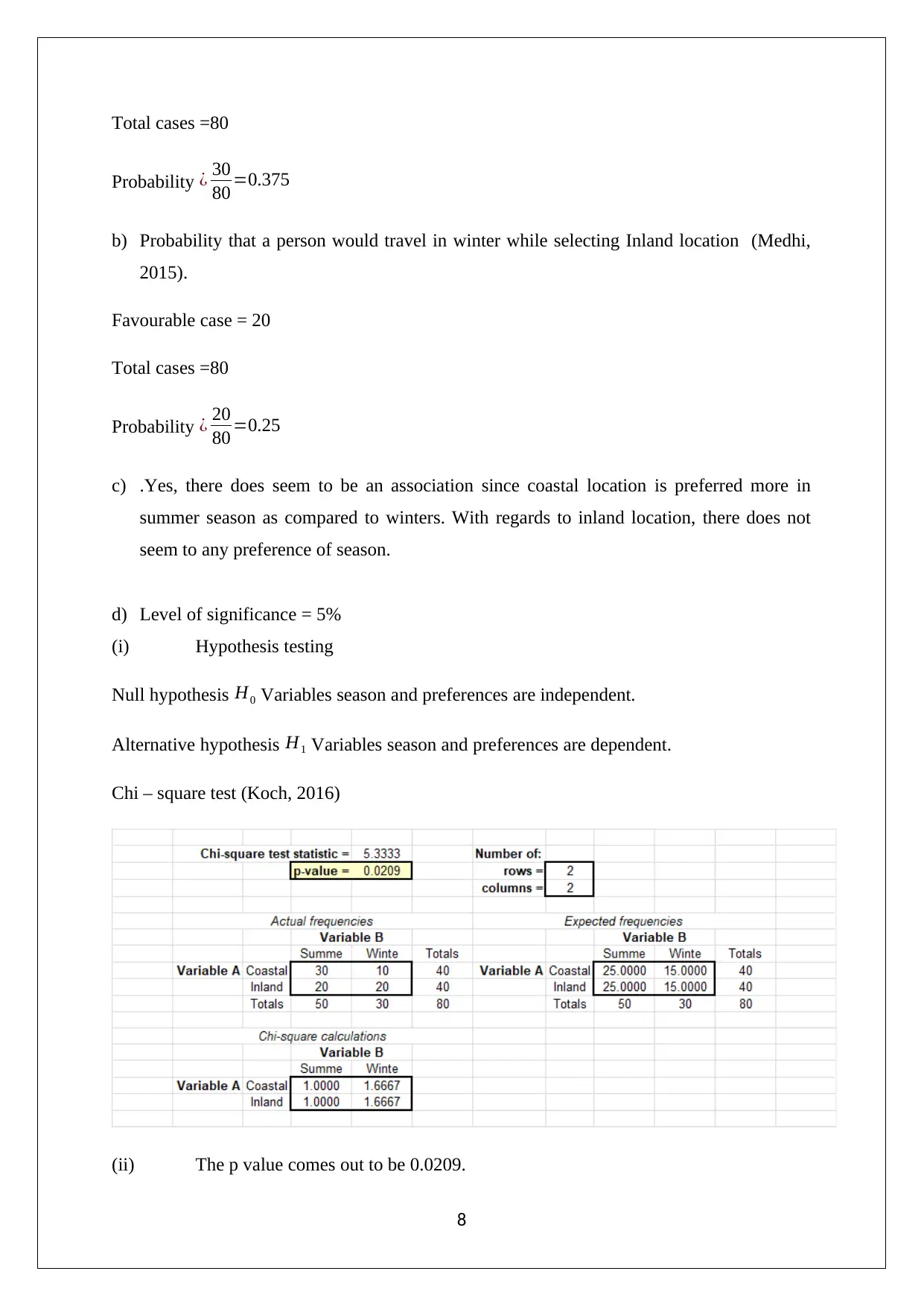
This assignment solution focuses on applying statistical analysis to support decision-making, covering topics from data types and graphical representations to hypothesis testing. It addresses questions related to identifying variable types, creating appropriate graphs (like bar charts and histograms), and interpreting statistical results. The solution includes analysis of lost-time injury causes, weight distribution of ball packets, and client satisfaction survey scores. Hypothesis testing is performed to determine if the average satisfaction score differs from a hypothesized value and whether there's a difference in satisfaction levels between large and small clients. The assignment also explores the association between travel season and preferred location using pivot tables and chi-square tests. The final recommendation emphasizes the importance of aligning project manager incentives with client satisfaction levels, irrespective of client size. Desklib offers a wealth of similar solved assignments and past papers for students.

S A S CA A A S S S R D C S MAT TI TI L N LY I TO UPPO T E I ION KING
Student d ameI / N
[Pick the date]

Question 1
a) Cause is a nominal variable since it presents a series of labels which cannot be arranged
in any logical order. If on the other hand, the labels could have been independently
expresses in a logical sequence, then the variable would have been ordinal but this is not
the case here.
b) The appropriate graph is bar chart.
c) Bar chart to represent the data
Vehicle Accident
all slip on same levelF /
all from heightF
it by falling objectH
ushing pulling objectP /
Contact with chemical
Cut by tools
posed to mental stressEx
ther mechanismsO
0 5 10 15 20 25 30 35
4
25
3
31
5
5
14
4
9
Bar Chart
%
Cause
d) From the above chart, it is apparent that the most common cause of lost-time injury at the
mining site has been through hit by a falling object. Other likely cause of lost-time injuries
include same level fall or slip and also being cut by tools. Together, these three causes
contribute to about 60% of the lost-time injuries incurred at the mining site. The other causes
have relatively low incidence and thus, these major causes must be contained (Lehman &
Romano, 2016).
Question 2
(a) Graphical display of distribution
Mean = 300 grams
1

Standard deviation σ =10 grams
(b) Company has the requirement of packets of balls of weight at least 280 grams.
(i) Graph
2

(ii) The understanding of the empirical rule can be highlighted using the following diagram.
In this case, since μ = 300g and σ = 10g, hence the rejected region would have a probability
of 0.025.
c) 290 g is indicative of μ- σ while 330g is indicative of μ+ 3σ
The % of data lying between μ- 3σ and μ+3σ in accordance with the empirical rule is 99.7%.
However, in order to obtain the answer for the given part, suitable deductions need to be
made for the area between μ- σ and μ- 3σ (Lehman & Romano, 2016).
% values lying between μ- 3σ and μ- σ = 13.5% + 2.5% -[(100-99.7)/2]% = 15.85%
Hence, required probability = 0.997-0.1585 = 0.8385
3

Question 3
(a) Graphical display of survey score
0 - 16 16 - 30 30- 44 44 -58 58 - 72 72 -86 86 -100
0
10
20
30
40
50
60
70
80
90
Histogram : Survey Score
Survey Score
Freuqnecy
(b) It is apparent from the above graph that the tail on the left side is longer than the one
on the right which is indicative of the presence of negative skew (Shi & Tao, 2015).
Since one of the key requirements of normal distribution is that the symmetric
alignment of the normal curve, clearly the given distribution is not normal.
(c) Summary statistics
4

As negative skew is present along with potential outlier values speciality on the lower end,
hence mean might be distorted to indicate a lower value. Thus, central tendency for the given
data would be best represented using median which is not impacted by extreme values on
either sides. Further, in relation to deviation, standard deviation may not be reliable and
hence IQR or Inter-Quartile Range may be preferred (Shi & Tao, 2015).
(d) (i) Hypothesis testing
Null hypothesis H0 : μ=55
Alternative hypothesis H1 : μ ≠55
(ii) The value of sample mean from the above shown descriptive statistics comes out to be
59.62. Hence, it can be said that values of sample mean and the hypothesized mean are
similar.
(iii) The value of t stat ¿ x−μ
S . E . = 59.62−55
1.19 =3.90
(iv) The p value would be calculated as =1-T.DIST(3.90,299,TRUE) which comes out to be
0.0001.
(v) It can be seen that p value is lower than level of significance (0.02<0.05) and therefore,
null hypothesis would be rejected and alternative hypothesis would be accepted (Medhi,
2015).
(vi) It can be concluded that the average satisfaction survey score of clients is not 55.
Question 4
(a) (i) Graphical display
5

(ii) The key difference as apparent from the above graph is that a higher satisfaction score is
witnessed for larger clients in comparison to smaller clients. A key similarity is that majority
of the satisfaction survey scores for both big and small clients are concentrated in the middle
values with limited concentration in the extremes (Lind, Marchal & Wathen, 2016).
(b) Level of significance = 5%
(i) Hypothesis testing (Harmon, 2015)
Null hypothesis H0 : μSmaller clients=μLarger clients
6

Alternative hypothesis H1 : μSmaller clients ≠ μLarger clients
(ii) The two tailed p value comes out to be 0.02.
(iii) It can be seen that p value is lower than level of significance (0.02<0.05) and therefore,
null hypothesis would be rejected and alternative hypothesis would be accepted (Lehman &
Romano, 2016).
(iv) It may be concluded that the satisfaction level across the big clients and small clients
tends to differ which may be indicative of potential differential in providing service to these
two groups.
(v) Management needs to link the incentive of project managers with the satisfaction level of
clients irrespective of their underlying size. This would ensure that proper attention and
customer service would be extended to both big and small clients.
Question 5
Pivot table
a) Probability that a person would travel in summer while selecting Coastal location.
Favourable case = 30
7

Total cases =80
Probability ¿ 30
80 =0.375
b) Probability that a person would travel in winter while selecting Inland location (Medhi,
2015).
Favourable case = 20
Total cases =80
Probability ¿ 20
80 =0.25
c) .Yes, there does seem to be an association since coastal location is preferred more in
summer season as compared to winters. With regards to inland location, there does not
seem to any preference of season.
d) Level of significance = 5%
(i) Hypothesis testing
Null hypothesis H0 Variables season and preferences are independent.
Alternative hypothesis H1 Variables season and preferences are dependent.
Chi – square test (Koch, 2016)
(ii) The p value comes out to be 0.0209.
8

(iii) It can be seen that p value is lower than level of significance and therefore, null
hypothesis would be rejected and alternative hypothesis would be accepted (Lind,
Marchal & Wathen, 2016).
(iv) Conclusion can be drawn that the underlying season does influence the preferred
location of people to visit.
(e) During winters, it is apparent that people tend to visit both inland and coastal locations
and hence both need to be advertised. This is not the case in summers when coastal locations
have a clear edge.
9

References
Harmon, M. (2015) Hypothesis Testing in Excel - The Excel Statistical Master (7th ed.).
Florida: Mark Harmon.
Koch, K.R. (2016) Parameter Estimation and Hypothesis Testing in Linear Models (2nd ed.).
London: Springer Science & Business Media.
Lehman, L. E. & Romano, P. J. (2016) Testing Statistical Hypotheses (3rd ed.). Berlin :
Springer Science & Business Media.
Lind, A.D., Marchal, G.W. & Wathen, A.S. (2016) Statistical Techniques in Business and
Economics (15th ed.). New York : McGraw-Hill/Irwin.
Medhi, J. (2015) Statistical Methods: An Introductory Text (4th ed.). Sydney: New Age
International.
Shi, Z. N. & Tao, J. (2015) Statistical Hypothesis Testing: Theory and Methods (6th ed.).
London: World Scientific.
10