Statistical Analysis for Managerial Decisions: Assignment 2

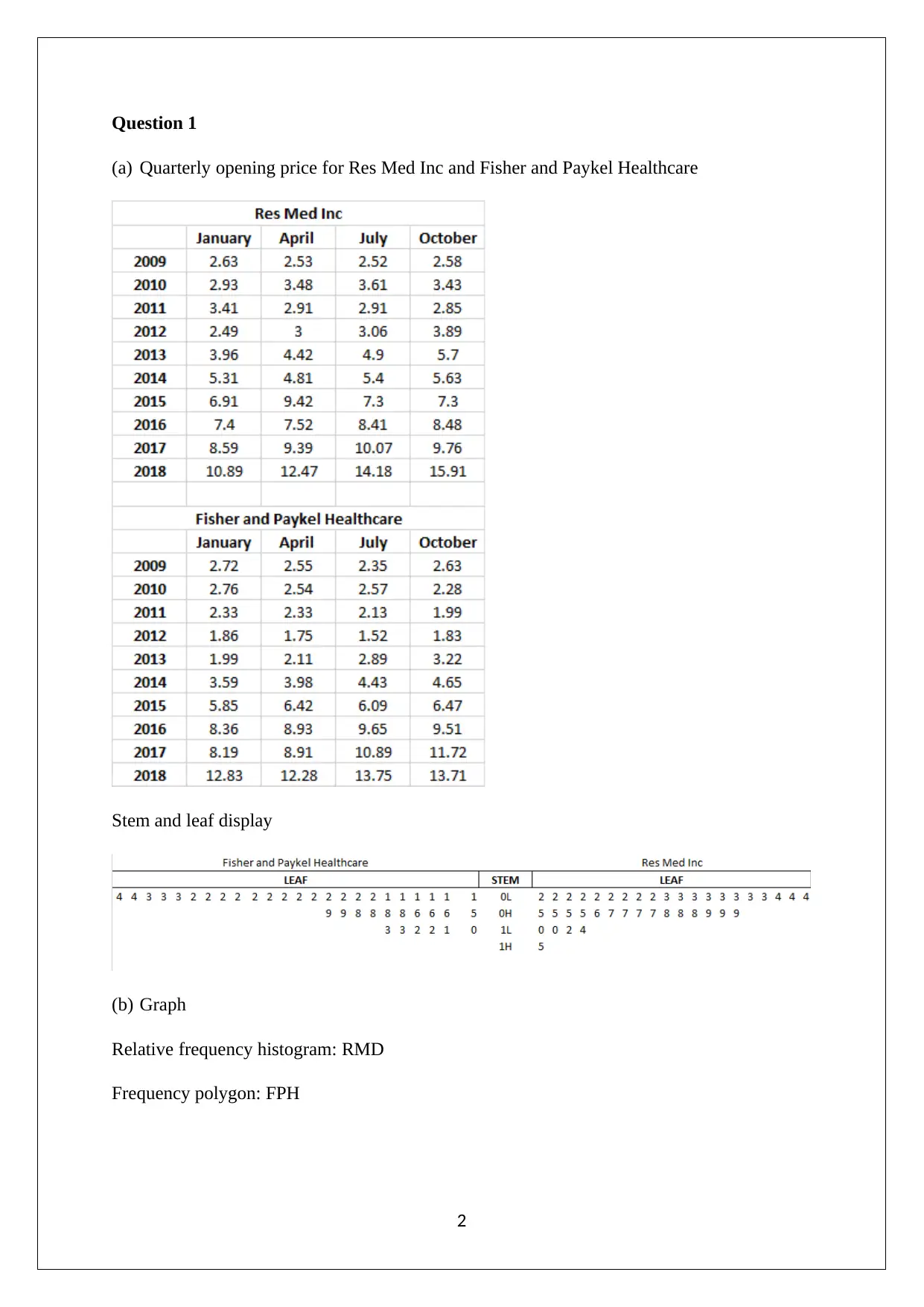
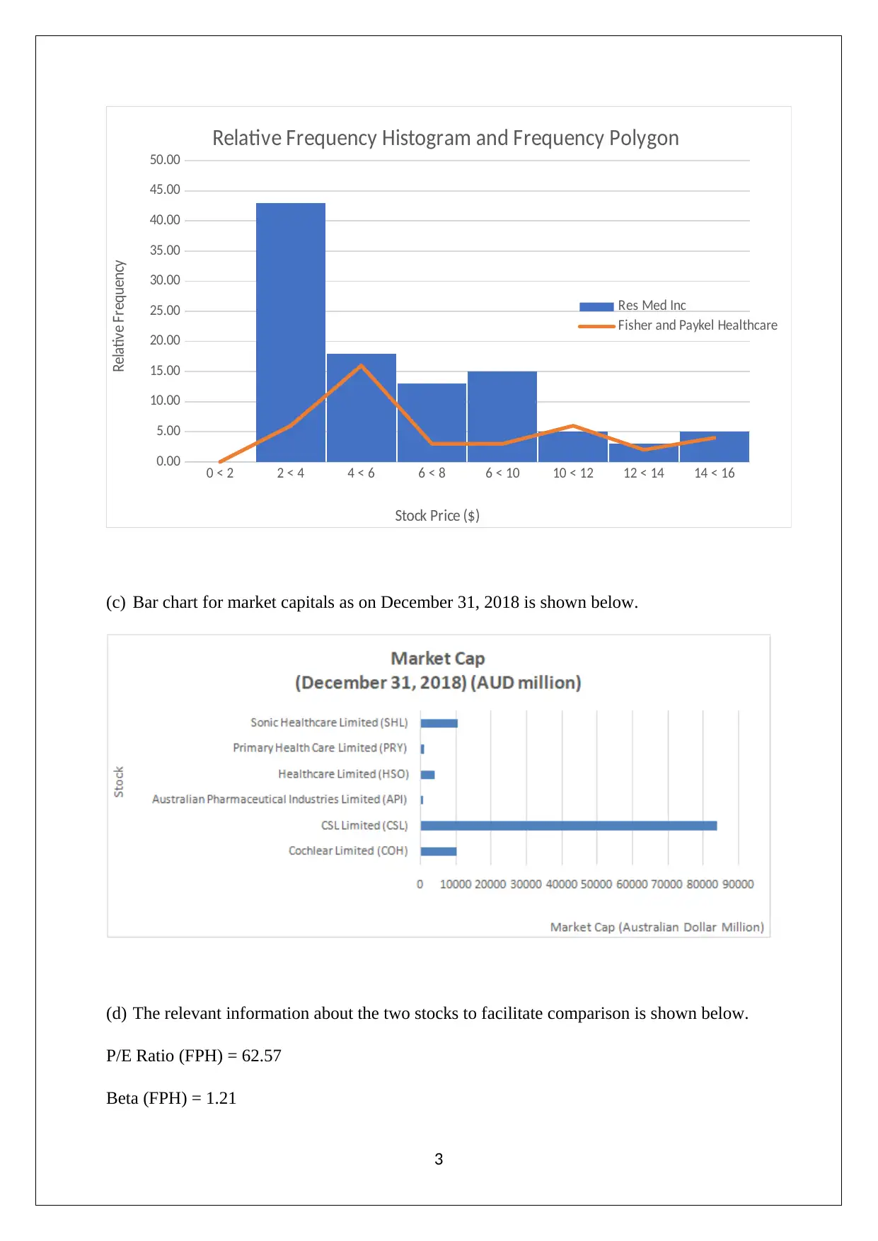
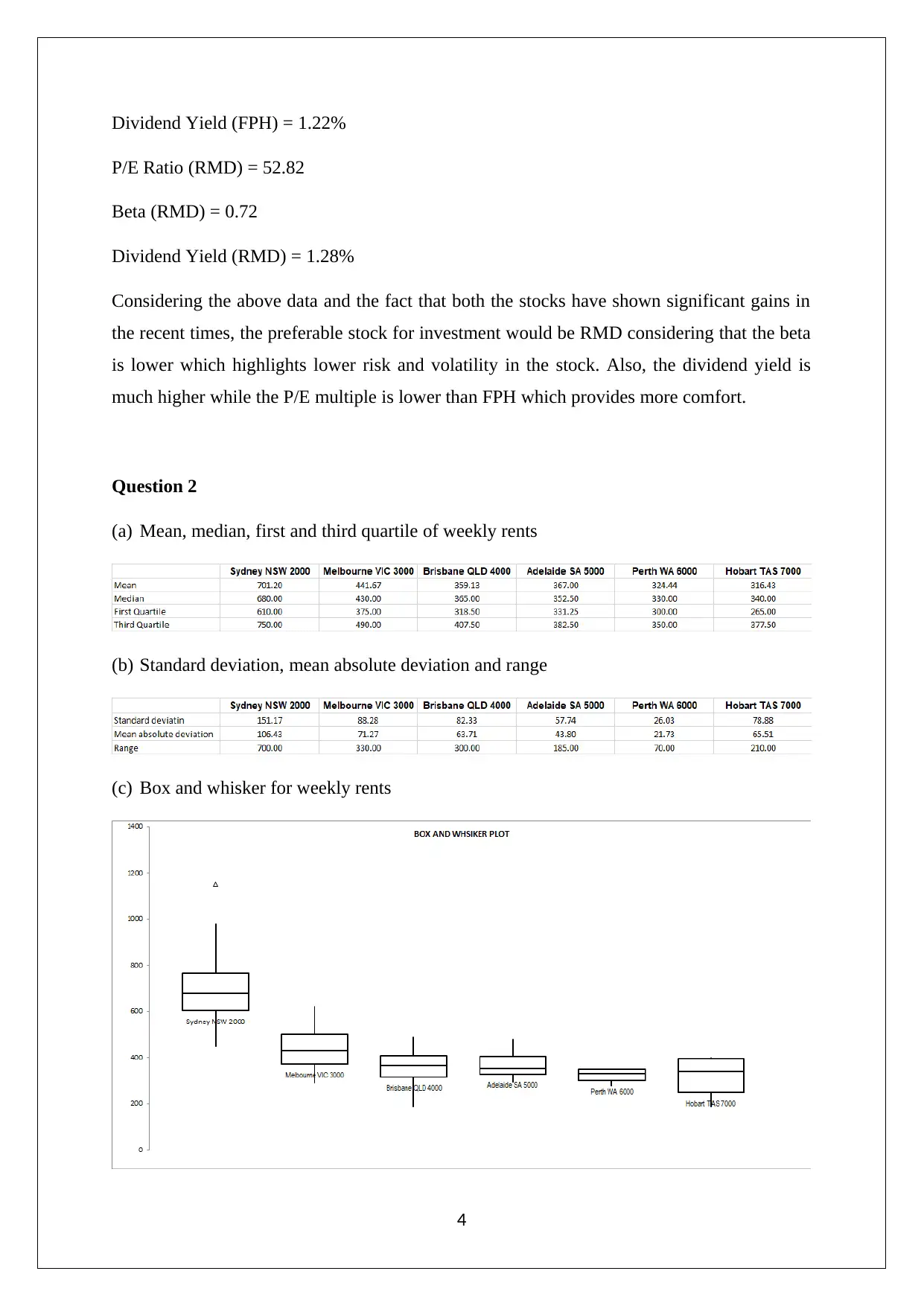
This assignment solution provides a comprehensive analysis of statistical concepts applied to managerial decision-making. It includes topics such as descriptive statistics, probability distributions (Poisson and Normal), confidence intervals, and comparative stock analysis. The solution uses real-world examples like stock prices, weekly rents, and rainfall data to illustrate the application of statistical methods. The analysis covers stem and leaf displays, histograms, bar charts, and box-and-whisker plots for data visualization. Probability calculations, including Poisson and Normal distributions, are performed to assess the likelihood of various events. Confidence intervals are constructed and interpreted to determine significant differences between groups. The assignment also evaluates the reliability of statistical estimates based on standard errors. References to relevant statistical literature are provided to support the methods used.

STATISTICS FOR MANAGERIAL DECISIONS
STUDENT ID:
[Pick the date]

Question 1
(a) Quarterly opening price for Res Med Inc and Fisher and Paykel Healthcare
Stem and leaf display
(b) Graph
Relative frequency histogram: RMD
Frequency polygon: FPH
2

0 < 2 2 < 4 4 < 6 6 < 8 6 < 10 10 < 12 12 < 14 14 < 16
0.00
5.00
10.00
15.00
20.00
25.00
30.00
35.00
40.00
45.00
50.00
Relative Frequency Histogram and Frequency Polygon
Res Med Inc
Fisher and Paykel Healthcare
Stock Price ($)
Relative Frequency
(c) Bar chart for market capitals as on December 31, 2018 is shown below.
(d) The relevant information about the two stocks to facilitate comparison is shown below.
P/E Ratio (FPH) = 62.57
Beta (FPH) = 1.21
3

Dividend Yield (FPH) = 1.22%
P/E Ratio (RMD) = 52.82
Beta (RMD) = 0.72
Dividend Yield (RMD) = 1.28%
Considering the above data and the fact that both the stocks have shown significant gains in
the recent times, the preferable stock for investment would be RMD considering that the beta
is lower which highlights lower risk and volatility in the stock. Also, the dividend yield is
much higher while the P/E multiple is lower than FPH which provides more comfort.
Question 2
(a) Mean, median, first and third quartile of weekly rents
(b) Standard deviation, mean absolute deviation and range
(c) Box and whisker for weekly rents
4

(d) It is quite evident that there is significant difference in the average advertised weekly
rents for 1 bed 1 bath apartment in various Australian cities. As expected highest weekly
rents are observed for Sydney while the lowest is observed for Perth. With regards to
Melbourne also, the average weekly rent is about $ 35 lower than the average mean rent
for apartment in Sydney. The given rates are significantly higher than the corresponding
weekly rents available at the current places through Airbnb. In most of the locations such
as Sydney and Melbourne, the listings are available are lower rent values then the above
mean.
Question 3
(a) Probability that the a randomly picked crop field would be canola field in Australia
(Hillier, 2016)
P ( Canola field ) = 2538678
(4623527+2538678+ 371339+ 955321+11720277) =0.1256
(b) Probability that the a randomly picked crop field would be Wheat field in NSW
P ( Wheat field ) = 9556517
(2755310+ 1201045+ 403121+483081+9556517) =0.6637
(c)Yield of Barley( Aust .)= Production
Area =12920461
4623527 =2.795
Yield of Barley(NSW )= Production
Area =2755310
1008269 =2.733
Yield of Barley (VIC )= Production
Area =3100466
954176 =3.249
Yield of Barley(QID )= Production
Area = 413023
141960 =2.909
Yield of Barley(SA)= Production
Area = 2744507
922787 =2.974
5

Probability that barley grown in SA ¿ 2.974
2.733+3.249+2.909+2.974 =0.251
(d)The grain sorghum estimates for South Australia (SA) would be considered as unreliable
because of the underlying standard error being more than 50%.
Question 4
(a) Poisson distribution
(i) Probability that on any week there is no rainfall
Number of days in a year on which rainfall was incurred = 170
Mean number of days on which rainfall was incurred = 170/52 = 3.3077
No rainfall means X = 0
Now,
P( X=0∨λ=3.3077)=3.30770 × e−3.30779
0!
P( X=0∨λ=3.3077)=0.0366
(ii) Probability that there will be 3 days or more than 3 days of rainfall in a week
Rainfall 3 days or more than 3 days means X >= 3
Now,
P( X ≥ 3∨ λ=3.3077)=1− 3.30773 × e−3.30779
3! =1−0.5786
P( X ≥ 3∨ λ=3.3077)=0.4214
(b) Normal distribution
Mean amount of rainfall = 83.75 mm per week
Standard deviation of amount of rainfall = 152.74 mm
6

Standard error = Standard deviation
√ (52 ) =21.18
(i) Probability that in a given week there is rainfall between 10 mm and 50 mm of
rainfall (Fick, 2015)
Z 1= X 1−mean
Standarderror = 10−83.75
21.18 =−3.48
P ( Z 1<−3.48 )=0.000249
Z 2= X 2−mean
Standarderror = 50−83.75
21.18 =−1.59
P ( Z 2<−1.59 ) =0.055526
Hence,
P ( 10< X <50 )=P ( Z 2<−1.59 )−P ( Z 1<−3.48 )
P ( 10< X <50 )=0.055526−0.000249=0.055277
Hence, there is 0.05527 probability that in a given week there is rainfall between 10 mm and
50 mm of rainfall.
(i) Amount of rainfall when only 12% of weeks have that amount of rainfall or higher
P ( rainfall> x )=0.12
The z value for 12% can be found by using NORMSINV () excel function (Harmon, 2016).
z=NORMSINV ( 0.12 ) =−1.17499
Let the required amount of rainfall be X mm and hence,
z= X−mean
Standarderror
−1.17499= X −83.75
21.18
X =58.86 mm
7

Therefore, the amount of rainfall when only 12% of weeks have that amount of rainfall or
higher would be 58.86 mm.
Question 5
(a) Normality plot of the variables is shown below.
80 100 120 140 160 180 200 220
-4
-3
-2
-1
0
1
2
3
4
Normal Probability Plot
Resting Blood Pressure
Resting Blood Pressure
Zj
For the above variable, the distribution can be assumed as normal since there is a broad linear
pattern that is observed in the above plot (Hillier, 2016).
8

100 150 200 250 300 350 400 450 500 550 600
-4
-3
-2
-1
0
1
2
3
4
Normal Probability Plot
Serum Cholestoral in mg/dl
Serum cholestoral in mg/dl
Zj
For the above variable, the distribution can be assumed as normal since there is a broad linear
pattern that is observed especially if an outlier on the higher end is ignored.
60 80 100 120 140 160 180 200 220
-4
-3
-2
-1
0
1
2
3
4
Normal Probability Plot
Maximum Heart Rate Achieved
Maximum heart rate achieved
Zj
For the above variable, the distribution can be assumed as normal since there is a broad linear
pattern that is observed in the above plot.
9

0 1 2 3 4 5 6 7
-4
-3
-2
-1
0
1
2
3
4
Normal Probability Plot
Old Peak= ST Depression Induced by Exercise Relative to
Rest
Old peak =ST Depression induced by exercise relative to rest
Zj
For the above variable, the distribution can be assumed as normal since there is a broad linear
pattern that is observed especially if couple of outliers on the upper and lower end are ignored
(Fehr and Grossman, 2013).
(b) 90% confidence interval for the variables for the patients with heart disease and without
heart disease
Absence heart disease Presence heart disease
10

11

Significant difference between the patients with and without heart disease would be observed
for those variables where there is no overlapping of the 90% confidence interval determined
above (Medhi, 2016). These variables are as indicated below.
1) Resting blood pressure
2) Oldpeak
3) Maximum heart rate achieved
12