Statistical Analysis Exam Solution for MAT10251 at SCU

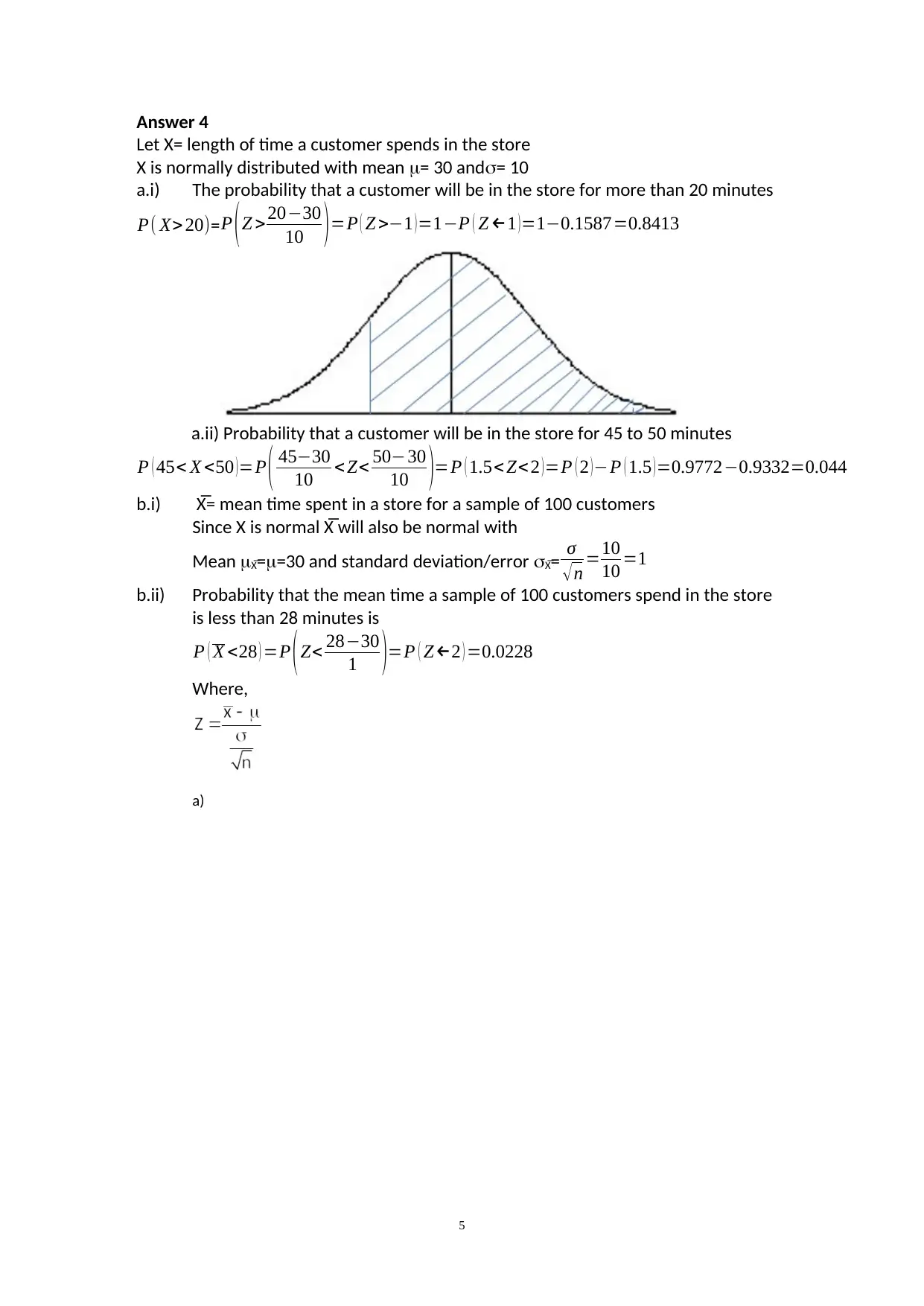
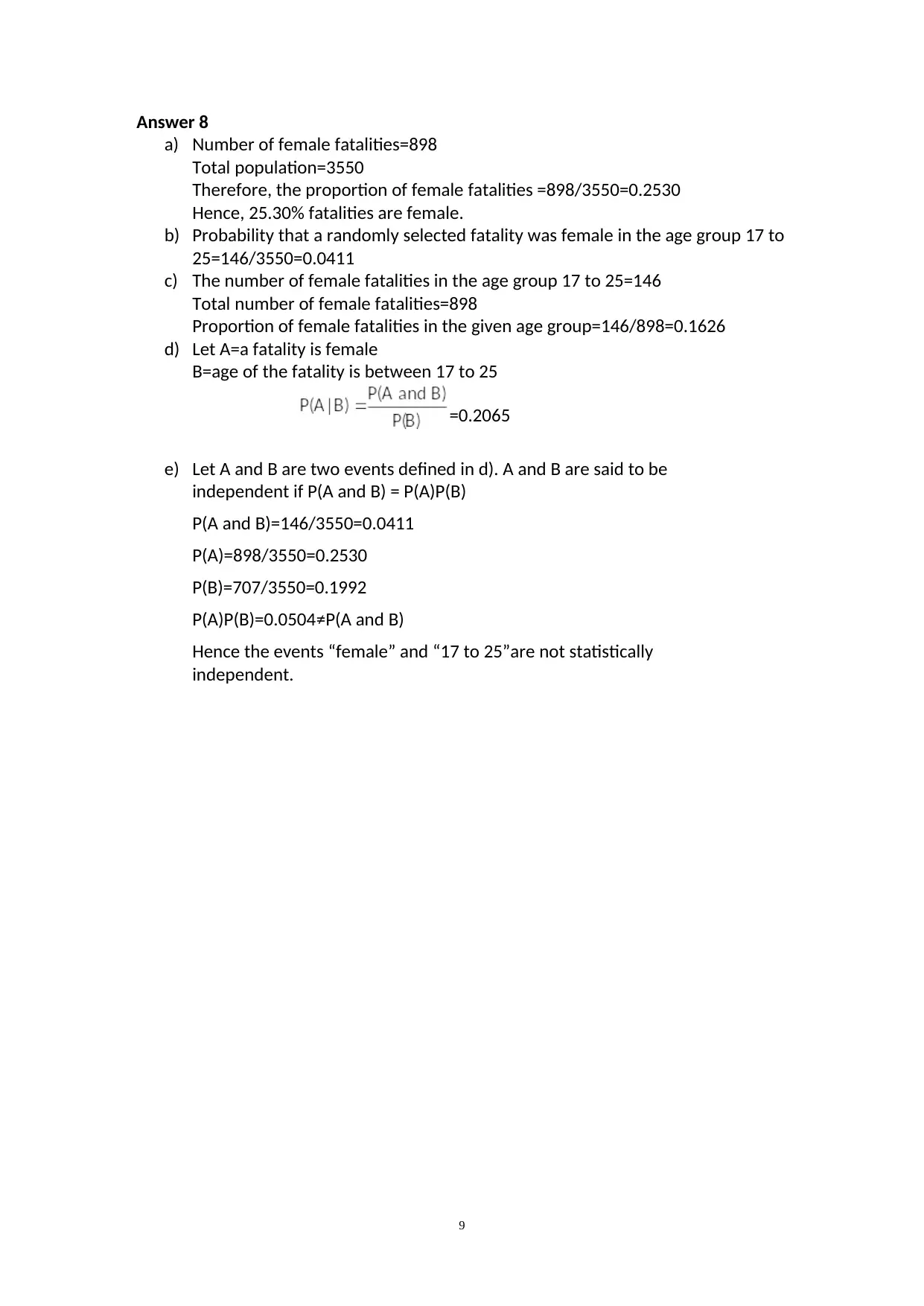
This document presents a complete solution to the MAT10251 Statistical Analysis exam administered by Southern Cross University. The exam covers a wide range of statistical concepts, including descriptive statistics, hypothesis testing, confidence intervals, and regression analysis. The solution provides detailed answers to each question, demonstrating the application of statistical methods to real-world scenarios. Topics covered include the analysis of call center data, the probability of customer behavior, and the relationship between advertising expenditure and sales. The solution also addresses multiple regression analysis and the independence of events, providing a comprehensive overview of the statistical techniques required for the course. The exam solution is a valuable resource for students preparing for similar assessments, offering insights into problem-solving approaches and statistical reasoning.

SOUTHERN CROSS UNIVERSITY
School of Business and Tourism
MAT10251 Statistical Analysis
EXAM COVER SHEET
Please complete all of the following details and then make these sheets the first page
of your exam.
Your exam must be submitted in one of the following formats: Word (docx), PNG or JPG.
Student Name: ANKIT KHANAL
Student ID No.: 23255155
Declaration:
I have read and understand the Rules Relating to Awards (Rule 3 Section
18 – Academic Integrity) as contained in the SCU Policy Library. I
understand the penalties that apply for academic misconduct and agree
to be bound by these rules.
The work I am submitting electronically is entirely my own work.
.
Signed:
(please type
your name)
Ankit Khanal
Date: 14.04.2020

Answer 1
a) i) The histogram shows that the number of received calls variers from 45
to 125 over a four week period. In other words, the number of calls is
approximately between 50 to 120.
ii) Since the histogram is mount shaped and approximately symmetric it
can be deduced that the distribution of number of call received is
approximately normal, with center in the modal class 80 to 90.
b) I) Mean: x̅=85, Standard deviation: s=13.2539
ii) Median is Md= n+1
2 = 26
2 =13 th ranked value
Median:Md= x12+ x13
2 =85
Q1= n+1
4 = 26
4 =6.5 thranked value
Q1=75
Q1= 3 ( n+1 )
4 = 3 x 26
4 =19.5 th ranked value
Q3=92
iii) mode= 85, Range=max(x)-min(x)=111-59=52.
2

Answer 2
Let X=number of calls per hour
=mean number of calls per hour
From question 1, mean: x̅ =85, n=25, s=13.2539
To test ,
H0: 80
H1:>80
Since the population standard deviation is unknown and X is approximately normal
Test Statistic: T =x− ¿
s
√n
withdf =n−1 ¿
Level of significance: α=0.1
Critical value:tα ,24=1.317 8
Reject the null hypothesis if T>1.3178 otherwise accept it.
Here T=1.8862
T>1.378, hence the null hypothesis is rejected at 10% level.
Therefore at 10% level, the average number of calls per hour is greater than 80.
Hence, it is suggested that the call centre should increase their staffing levels.
3

Answer 3
a) There are 9 observations where more than 90 calls were received.
Sample proportion p= 9
25 =0.36
b) Let π=proportion of hours with more than 90 calls received.
Given n=25, p=0.36
Since np=9 and n(1-p)=16>5, sampling distribution of P is approximately
normal, so no assumptions are required.
CI for proportion p ± zα /2 √ p(1− p)
n
For 95% CI, α =0.05 , z α
2
=z0.025=1.96
95% CI for π is
0.36 ± 1.96 √ 0.36(1−0.36)
25 =0.36 ± 0.18816= ( 0.17184,0.54816 ) .
It can be concluded with 95% confidence that between 17.18% and 54.82%
hours , the number of calls is more than 90.
4

Answer 4
Let X= length of time a customer spends in the store
X is normally distributed with mean = 30 and= 10
a.i) The probability that a customer will be in the store for more than 20 minutes
P( X> 20)=P (Z >20−30
10 )=P ( Z >−1 )=1−P ( Z ←1 )=1−0.1587=0.8413
a.ii) Probability that a customer will be in the store for 45 to 50 minutes
P ( 45< X <50 )=P ( 45−30
10 < Z< 50−30
10 )=P ( 1.5< Z< 2 )=P ( 2 )−P ( 1.5 )=0.9772−0.9332=0.044
b.i) X̅= mean time spent in a store for a sample of 100 customers
Since X is normal X̅ will also be normal with
Mean X̅==30 and standard deviation/error X̅= σ
√n =10
10 =1
b.ii) Probability that the mean time a sample of 100 customers spend in the store
is less than 28 minutes is
P ( X <28 ) =P (Z< 28−30
1 )=P ( Z←2 ) =0.0228
Where,
a)
5

Question 5
a) The distribution of travel time to school in Queensland is skewed to the left
whereas that for in New South wales is slightly skewed to the right. Therefore,
the distribution of travel time to school for both Queensland and New South
Wales cannot be considered to be approximately normal.
b) Different students were taken for two different samples. Hence the samples
are independent.
c) Let
XQ= Travel time to school in Queensland
XN=Travel time to school in New South Wales
Q= mean travel time to school in Queensland
N= mean travel time to school in New South Wales
Since the samples are large and XQ and XN are not extremely skewed, a t-test
can be used.
The population standard deviations Q and N are unknown but assumed to be
equal. Since the standard deviations of the sample do not differ much, a
pooled variance t-test can be used.
In other way,
XQ and XN are not normal, however as large samples are taken the sampling
distribution of X̅ Q - X̅ N is approximately normal, according to Central Limit
Theorem. Hence z-test can be applied. The population standard deviations Q
and N are unknown which can be estimated by the sample standard
deviations sQ and sN.
d) Level of significance: α=0.1
To test
H0: Q =N (no difference)
H1: Q ≠N (difference)
Decision: Since the test statistic is 0.6683<1.6449 ( or p-value=0.5039>0.1
level of significance) the null hypothesis is not rejected at 10% level of
significance.
Conclusion: It can be concluded that there is no significant difference in
average travel time to school in Queensland and New south Wales, at 10%
level of significance.
6

Answer 6
a) The scatterplot shows that there is a strong positive relationship between
weekly advertising expenditure and weekly sales.
b) Let,
X= Weekly advertising expenditure (independent variable)
Y= Weekly sales, 000$ (dependent variable)
The least square regression line is,ŷ
=b 0+b1x5.208+29.674x
c) The gradient of the regression line b1=29.674
This means that if the weekly expenditure is increased by one unit, then the
weekly sales will b increased by 29.674 units that is 29674$.
d) Given x=4500ŷ
=5.208+29.674*4500=133538.208
e) The coefficient of determination r2=0.590.
Approximately 59% variability in weekly sales can be explained by its linear
relationship to weekly advertising expenditure.
7

Answer 7
a) Let D= Direct mail
T=Local Television
O=Online
S=Weekly sales
The multiple regression equation is given as,
ŝ=47.620+11.205d+13.851t+18.966o
b) Coefficient of online : bO=18.966
This indicates that if the weekly expenditure on online advertising is increased
by one unit then the weekly sales will be increased by 18.966 units.
c) To test H0: βD=0 (direct mail is not significant)
H1: βD≠0 (direct mail is significant)
Level of significance: α=0.01
Decision:
As p-value (D)=0.3585>0.01, the null hypothesis is accepted H0: βD=0.
Hence, at 1% level of significance Direct Mail does not contribute
significantly to the model.
8

Answer 8
a) Number of female fatalities=898
Total population=3550
Therefore, the proportion of female fatalities =898/3550=0.2530
Hence, 25.30% fatalities are female.
b) Probability that a randomly selected fatality was female in the age group 17 to
25=146/3550=0.0411
c) The number of female fatalities in the age group 17 to 25=146
Total number of female fatalities=898
Proportion of female fatalities in the given age group=146/898=0.1626
d) Let A=a fatality is female
B=age of the fatality is between 17 to 25
=0.2065
e) Let A and B are two events defined in d). A and B are said to be
independent if P(A and B) = P(A)P(B)
P(A and B)=146/3550=0.0411
P(A)=898/3550=0.2530
P(B)=707/3550=0.1992
P(A)P(B)=0.0504≠P(A and B)
Hence the events “female” and “17 to 25”are not statistically
independent.
9