A Statistical Report on Gender Differences in Investment Behaviors

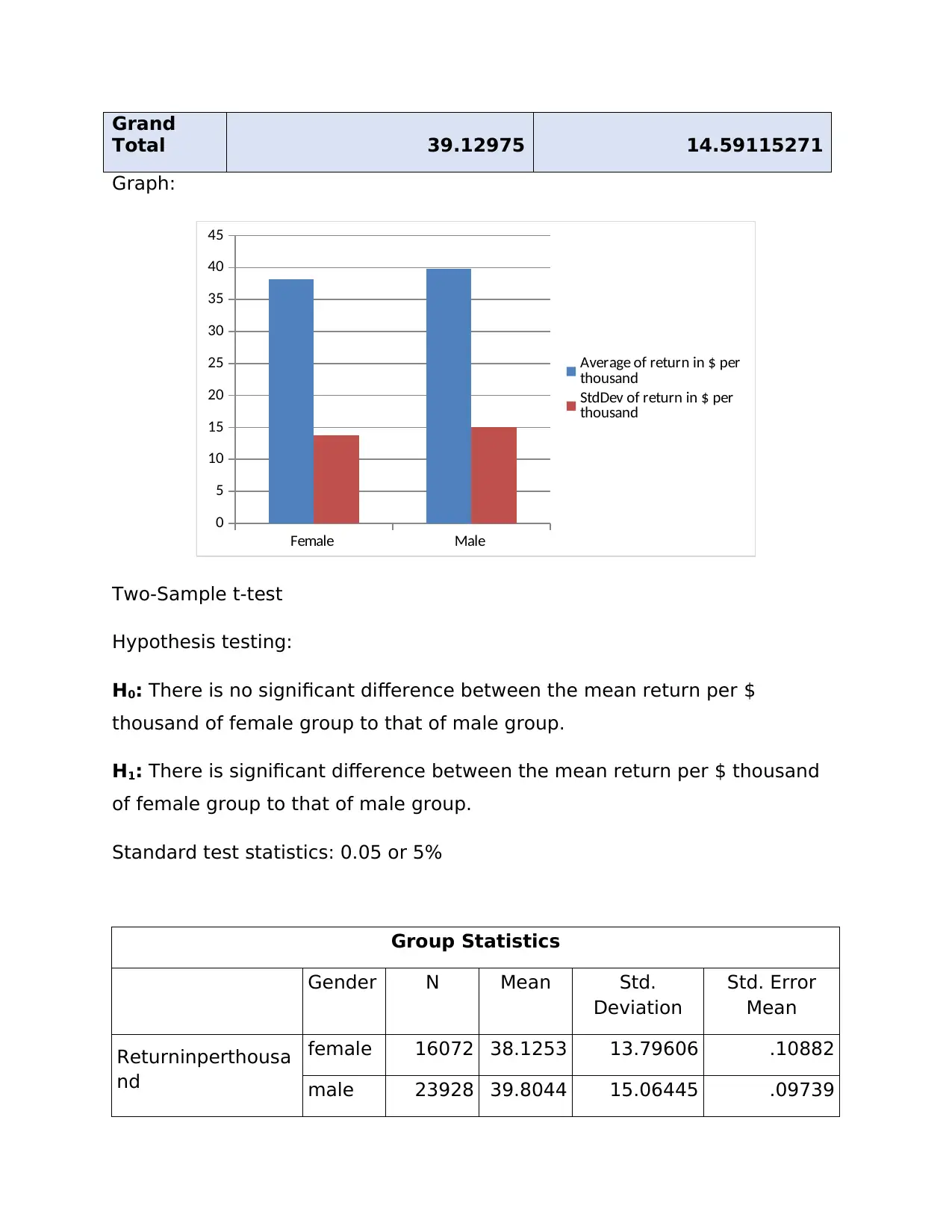
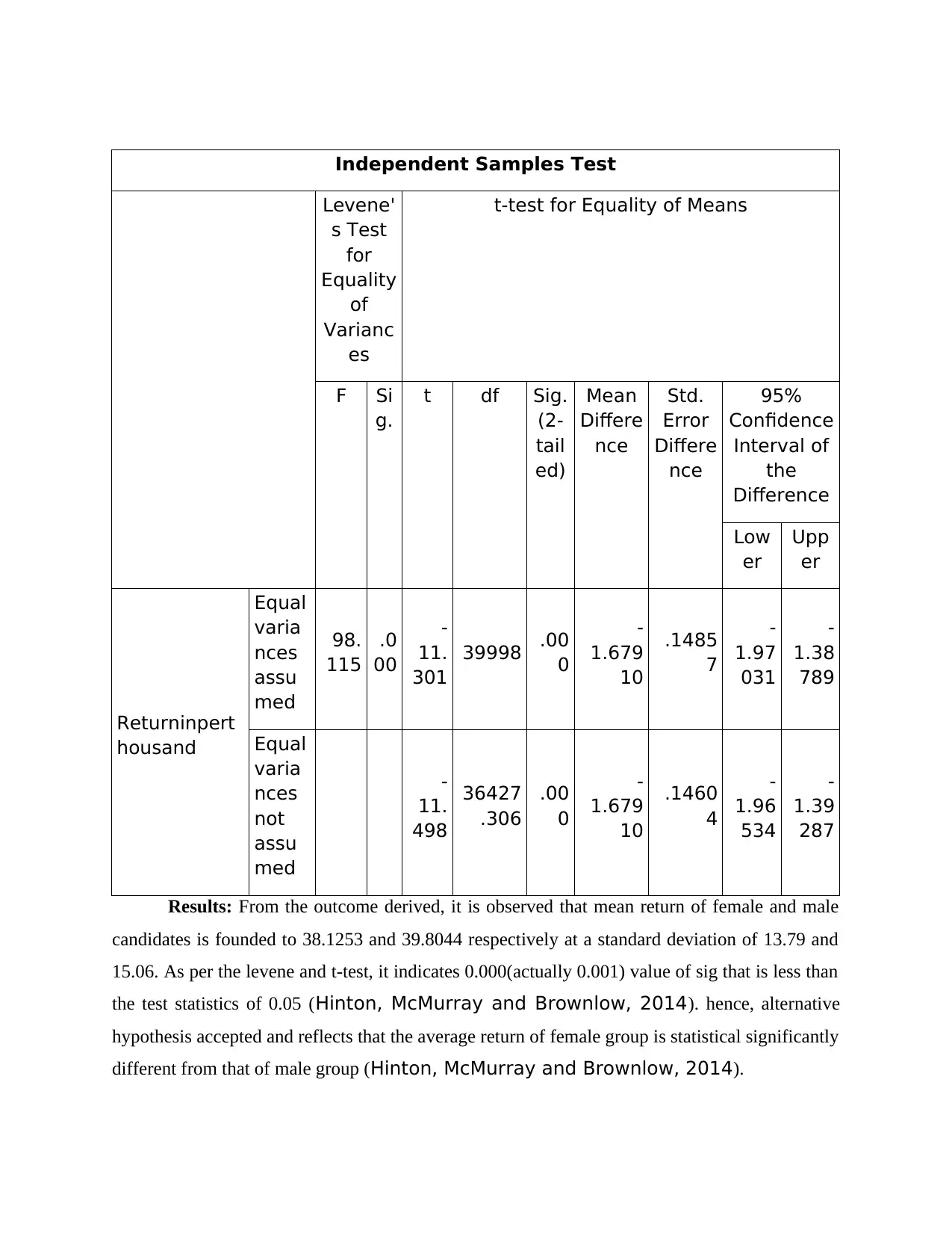
This report presents a statistical analysis of gender differences in investing, focusing on data from XYZ Investment Advisor. The analysis employs various statistical tools, including hypothesis testing, t-tests, and frequency tables, to evaluate investment behaviors and strategies. The report examines the preferences of male and female investors, comparing risk tolerance, investment types, and return rates. Findings indicate that while men tend to invest in higher-risk securities, women often make more informed investment decisions, leading to better returns. The analysis includes a chi-square test, t-test, and confidence intervals to assess the statistical significance of these differences. The conclusion suggests that new employees should focus on delivering strong returns and managing risk effectively, based on the insights derived from the statistical analysis. The report also highlights the importance of understanding consumer behavior and identifying opportunities for increased returns within the financial service industry.

Statistics

Table of Contents
INTRODUCTION...........................................................................................................................3
SECTION 2.....................................................................................................................................3
SECTION: 3....................................................................................................................................3
Option: 1......................................................................................................................................3
Option: 2......................................................................................................................................5
Option 3.......................................................................................................................................7
SECTION 4.....................................................................................................................................8
SECTION: 5....................................................................................................................................9
CONCLUSION..............................................................................................................................10
REFERENCES..............................................................................................................................11
Gender Differences in Investing:Shifting the Financial Services Industry.........................11

INTRODUCTION
Looking to the current uncertain market, decision-makers and
investors utilize number of statistical tools & models to deal with the
prospective uncertainities and changes in external conditions. Statistical
tools enable policy makers to make judgemental, realistic and convincing
decisions based on the statistical outcome. The aim of the given assignment
is to analyze & evaluate the investor database of XYZ investment advisor
which is an international organization and make investment on the behalf of
their consumers. In this, various statistical tests like hypothesis testing, t-test
and others along with the graphical visualization i.e. scatterplot and others
will be made for the purpose of making sound analysis.
SECTION 2
According to article males prefer to invest money in the securities high as compared to
females. The reason behind this, males are considered as risk taker and lays emphasis on taking
more risk with the motive to make value addition in the monetary aspects. Hence, it can be stated
that from evaluation that men tend to be highly overconfident in against to women (Gender
differences in investment: Shifting in the financial service sector, 2017).
Besides this, it has been found that men make more investment in terms of 45% over women.
Authors also mentioned in their report that trading reduces the return earned by men during a
year by 2.65. On the other side, such percentage accounts for 1.72% in the case of women. Thus,
it has been assessed that women are good investors in comparison to men. However, in the case
of excessive trading both men and women suffer high loss. Further, in article author stated that at
the time of making investment decision women consider several factors such as risk, return, time
period, credit rating of concerned organization etc (Male Investors vs. Female Investors, 2017).
On the other side, males make focus on generating higher returns by investing money in the
securities. Thus, it can be presented that females are smart investors as compared to males.

SECTION: 3
Option: 1
Two categorical variable:
I: Gender: Female/Male
II: Investment type: High risk/Low risk
Two-way frequency table
Crosstab
Gender Total
female male
Investment
type
high risk
Count 3564 7682 11246
Expected Count 4518.6 6727.4 11246.0
Low risk
Count 12508 16246 28754
Expected Count 11553.4 17200.6 28754.0
Total
Count 16072 23928 40000
Expected Count 16072.0 23928.0 40000.0
Interpretation: The derived outcome presented that female prefer low risk as their count
is derived to 12508 greater than the count of high risk to 3564. Likewise, male group is also
founded risk averse because the candidate with low investment risk is identified to 16246 greater
than that of risky group to 7682. Still, in comparison, the proportion of high risk is founded
higher for the male group (7682/23928*100) 32.10% while in female, it is (3564/16072*100)
22.18% only (Koch, 2013).
Chi-square test
Hypothesis testing
H0: The group of female with different investment type is independent to
male with high & low risk investment.

H1: The group of female with different investment type is not independent to
male with high & low risk investment.
Test statistics: 5% or 0.05
Chi-Square Tests
Value df Asymp.
Sig. (2-
sided)
Exact Sig.
(2-sided)
Exact Sig.
(1-sided)
Pearson Chi-Square 469.01
8a 1 .000
Continuity
Correctionb
468.52
6 1 .000
Likelihood Ratio 477.87
6 1 .000
Fisher's Exact Test .000 .000
Linear-by-Linear
Association
469.00
6 1 .000
N of Valid Cases 40000
Results: Sig. value is below the standard set (0.000>0.005) which accept the alternative
hypothesis by demonstrating that there is a relationship between investment type of both the
female and male group (Jaggia and et.al., 2016).
Option: 2.
Categorical variable: Gender: Female/Male
Numerical variable: Return in $ per thousand
Row
Labels
Average of return in $ per
thousand
StdDev of return in $ per
thousand
Female 38.1253111 13.79606397
Male 39.80441324 15.06444641

Grand
Total 39.12975 14.59115271
Graph:
Female Male
0
5
10
15
20
25
30
35
40
45
Average of return in $ per
thousand
StdDev of return in $ per
thousand
Two-Sample t-test
Hypothesis testing:
H0: There is no significant difference between the mean return per $
thousand of female group to that of male group.
H1: There is significant difference between the mean return per $ thousand
of female group to that of male group.
Standard test statistics: 0.05 or 5%
Group Statistics
Gender N Mean Std.
Deviation
Std. Error
Mean
Returninperthousa
nd
female 16072 38.1253 13.79606 .10882
male 23928 39.8044 15.06445 .09739

Independent Samples Test
Levene'
s Test
for
Equality
of
Varianc
es
t-test for Equality of Means
F Si
g.
t df Sig.
(2-
tail
ed)
Mean
Differe
nce
Std.
Error
Differe
nce
95%
Confidence
Interval of
the
Difference
Low
er
Upp
er
Returninpert
housand
Equal
varia
nces
assu
med
98.
115
.0
00
-
11.
301
39998 .00
0
-
1.679
10
.1485
7
-
1.97
031
-
1.38
789
Equal
varia
nces
not
assu
med
-
11.
498
36427
.306
.00
0
-
1.679
10
.1460
4
-
1.96
534
-
1.39
287
Results: From the outcome derived, it is observed that mean return of female and male
candidates is founded to 38.1253 and 39.8044 respectively at a standard deviation of 13.79 and
15.06. As per the levene and t-test, it indicates 0.000(actually 0.001) value of sig that is less than
the test statistics of 0.05 (Hinton, McMurray and Brownlow, 2014). hence, alternative
hypothesis accepted and reflects that the average return of female group is statistical significantly
different from that of male group (Hinton, McMurray and Brownlow, 2014).

Option 3
For option 3, income and amount invested are considered as numeric value which in turn
helps in assessing the extent to which
Particulars Income Amount invested
Mean 89897.95 172166
Standard deviation 3535.53 107478.8
The above depicted table shows that mean income level of 40000 respondents accounts for
89897.95. Further, standard deviation of income level is 3535.53 which show that in the near
future amount of income will deviate from such figures. Besides this, it has been assessed that
average amount invested by the respondents account for 172166. Further, figure of standard
deviation is 107478.78 respectively. Thus, it can be presented that according to income level
amount is invested by the individuals.
SECTION 4
Labels Count Average return
on per thousand
Standard
deviation on per
thousand
Grand total 40000 30 14.59
 N = 40000
 Mean value = 30
 Standard deviation = 14.59
 Standard error = 14.59 / square root of 40000
= 14.59 / 200
= 0.073
Upper confidence interval level

Mean value = +t * standard error
= 39.13 + 1.96 * 0.073
= 2.99 or 3
Lower interval confidence level
Mean value = - t * standard error
= 39.13 - 1.96 * 0.073
= 2.71
Assessing the extent to which mean value is above 30
H0: μ = 30
H1: μ > 30
(Mean value – μ) / (standard deviation /square root of n
= (39.13 – 30) / (14.59 / 200)
= 9.13 / 0.073
= 125
By considering the above aspect it can be presented that mean value is above 30. Thus,
alternative hypothesis is accepted and other one is rejected.
SECTION: 5
From the analysis carried above, it can be suggested to the new employees that XYZ
Investment Company is delivering good return to their consumers hence there is a probability of
success and progress in the near future. On the basis of the findings, new employees can be
advised to make rationalized investment of XYZ’s consumer’s money so that they can deliver
increased return to the users and exceed their satisfaction level (Pallant, 2013). They also can
be suggested to identify new investment opportunities wherein high return can be gained on the

investment. Besides this, they must encourage the consumers to take risk so that they can earn
high return in several investments; it helps to make them risk taker instead of risk averse
(Pallant, 2013).
CONCLUSION
By summing up this report, it has been concluded that females invest money in the
operations wisely. Further, it can be revealed from the report that significant difference takes
place in the value of high and low risk investments undertaken by males & females. Besides this,
it can be inferred that according to the income level males and females take decision in relation
to making investment.

REFERENCES
Books and Journals
Hinton, P.R., McMurray, I. and Brownlow, C., 2014. SPSS explained.
Routledge.
Jaggia, S. and et.al., 2016. Essentials of business statistics: communicating
with numbers. McGraw-Hill Education.
Koch, K.R., 2013. Parameter estimation and hypothesis testing in linear
models. Springer Science & Business Media.
Pallant, J., 2013. SPSS survival manual. McGraw-Hill Education (UK).
Online
Gender Differences in
Investing:Shifting the Financial Services Industry
Gender differences in investment: Shifting in the financial service sector. 2017. Online.
Available through: < http://gsm.ucdavis.edu/blog-feature/gender-differences-investing>.
[Accessed on 22nd May 2017].
Male Investors vs. Female Investors. 2017. Online. Available through: <
https://www.wsj.com/articles/male-investors-vs-female-investors-how-do-they-compare-
1430709406>. [Accessed on 22nd May 2017].