SCLG3702 Semester 2 Homework 1: Comparing Means and Statistical Tests

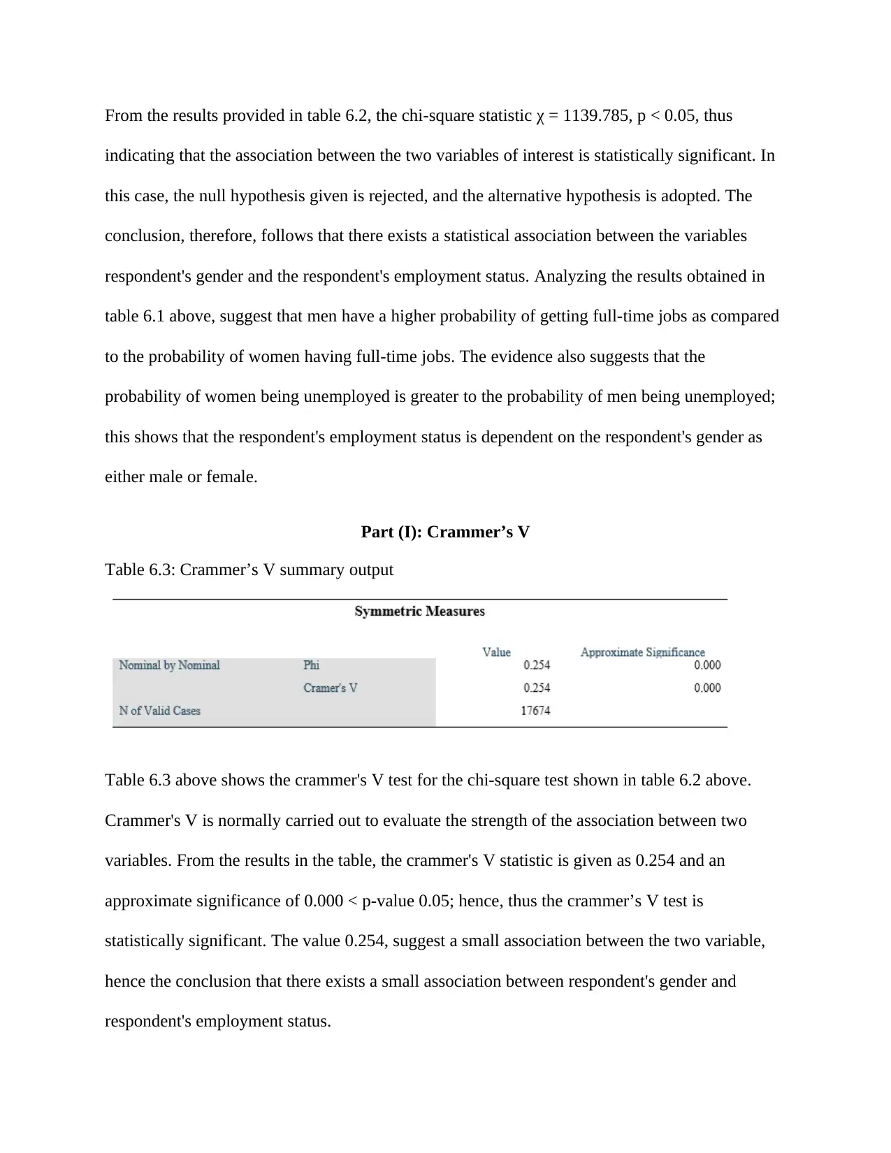
This homework assignment, titled "Homework 1," analyzes data from the HILDA survey to compare weekly income across different groups using various statistical methods. The assignment begins with a descriptive summary of weekly income, including measures of central tendency (mean, median) and dispersion (standard deviation, range, interquartile range), and assesses the skewness and kurtosis of the data. It then standardizes the weekly income data to calculate Z-scores and discusses the implications of these standardized values. The assignment also conducts conditional mean analysis to compare weekly income based on gender and performs one-sample and independent samples t-tests to test hypotheses about average weekly income and its relationship with gender. Finally, the assignment examines the association between gender and employment status using cross-tabulation, chi-square tests, and Cramer's V to evaluate the strength of the association. The analysis reveals differences in income and employment patterns between men and women, providing insights into potential disparities.

Comparisons of Means
Name
Professor
Institution
Date

Part (A) Descriptive summary for weekly income
Descriptive statistics consist of measures that describe the nature of the data, and these measures
include measures of central statistical measures and measures of dispersion. Central measures
include the mean, median, and mode, while measures of variation include variance, standard
deviation, minimum, maximum, and range. Part one of this research project is meant to use
descriptive analysis to describe the weekly income wage.
Table 1.1: Descriptive summary for weekly income
Table 1.1 above shows the descriptive summary for weekly income. From the table, the average
weekly income for the respondent is 672.81 ± (7.512). The median weekly income is given as
250 significantly less than the mean weekly income, and the standard deviation for weekly
income is 972.643. The minimum weekly income recorded from the survey is zero dollars, while
the maximum weekly income recorded is 34523 dollars giving a weekly income range of 34523.

The interquartile range for weekly income is 1122. The 95% confidence interval for the mean
has an average lower bound for the weekly income of 658.07, and an average upper bound of
687.54. The results indicate that the average weekly income for the respondents in the survey lies
between 658 dollars and 687 dollars. Table 1.1 also shows that a skewness value of 5.821, which
is significantly greater than one hence indicating that the data is highly skewed. The kurtosis
value given as 133.02 is also too large and in this case, also indicates that the data present in the
variable weekly income is skewed, thus said not to follow the normal distribution curve. If the
data is skewed, it only suggests that it is not normally distributed with mean zero and standard
deviation one.
Part (B) Standard Values
Table 2.1: Descriptive summary for the standardized weekly income
Table 2.1 above shows a descriptive summary of the weekly income standardized values. The
minimum weekly income standardized value is recorded as -0.69173 while the maximum weekly

income standardized value is given as 34.80227, giving a range of 35.494. The mean weekly
income Z-score was obtained as 0.00 and a standard deviation of 0.00772 approximately.
Part (C): The Role of standardized values
A standard value also referred to as a Z- score, shows the number of standard deviations for
given measures in a variable from the mean. Standardization helps in identifying the exact
position of each observation in the variable within the distribution. For one to obtain a Z score,
the following mathematical steps are followed
 Obtain the following statistical measures; the mean and the standard deviation for the
variable distribution
 Obtain the difference of each variable observation, and the sample means provided for
the data.
 Divide the results obtained above with the standard deviation for the data distribution.
Z scores give the parameters of a normal distribution of mean zero and standard deviation. From
the results obtained above, the mean Z score for weekly income is approximately zero; however,
the standard deviation is less than one hence suggesting skewness in the distribution; thus,
weekly income wage does not follow a normal distribution.

Part (D) Conditional Means
Table 3.1: Conditional means for weekly income
The variables of interest for this test are weekly income and the gender status for the
respondents. Table 3.1 above shows the conditional means for weekly income categorized by
gender. From the analysis, male respondents have an average weekly income of 856.84 and a
standard deviation of 1177.352. Female respondents have an average weekly income of 505.88
and a standard deviation of 678.812. The table indicates that the male category consists of 7964
respondents, 816 less than female respondents who were recorded as 8780. From the results
provided, it is evident that male respondents have a higher weekly income wage as compared to
their female counterparts, hence suggesting that men get paid better as compared to women.
Part (E) One Sample Test
Table 4.1: Summary output one sample t-test
Table 4.1 above shows the summary output for a one-sample t-test for weekly income wage. The
variable of interest for the one-sample t=test is weekly income wage. The test is carried out with

the notion that the weekly income wage for the respondents is equal to 680 dollars. The test is
used to evaluate the following research hypothesis;
H0: The average weekly income wage for the respondents is equal to 680 dollars
H1: The average weekly income wage for the respondents is not equal to 680 dollars.
From the results obtained above the t-statistics t = -0.957, p = 0.339 > 0.05, indicating that the
test is statistically significant at 0.05 level of statistical significance. The null hypothesis given
for the research project is accepted, and the conclusion is given as, follows that the average
income is equal to 680 dollars. The results provided in part (A) above showed that the
confidence range for the average weekly income lies in the range 658.07 – 687.54, and 680 is
within this range; hence, the test is true.
Part (F) Independent samples t-test
Table 5.1: Independent samples t-test
Table 5.1 shows the independent samples t-test for weekly income wage and gender. The
response variable for the test is weekly income wage measured as a scale variable, while the
independent variable is the gender of the respondent, which is a nominal variable with two

possible responses male or female. The test is meant to evaluate the following research
hypothesis:
H0: There is no statistical association in the mean weekly wage for male respondents and the
average weekly income wage for female respondents.
H1: There is a statistical association for the mean weekly wage for male respondents and the
average weekly income wage for female respondents
The significance value for Levene’s test for equality is given as 0.000 < p, 0.05; hence, the test is
statistically significant with the assumption of the equality of variances among the responses.
The t-statistic t = 23.705, p < 0.05, and thus concluding that the test of association between the
two variables weekly income and gender statistically significant. The null hypothesis (H0), is
rejected as a 0.05 level of significance, and the alternative hypothesis (H1), is adopted for this
test. The conclusion for the test, therefore, follows that there is a difference in the average
weekly income wage for male respondents as compared to the weekly income wage for female
respondents. The results obtained above can be further explained by the results in table 3.1 above
for conditional means. The analysis shows that men respondents achieved a higher average
weekly income wage as compared to women respondents, hence suggesting a difference in the
weekly income wage for the two groups.

Part (G): Test for statistical association
Table 6.1: Cross-tabulation summary
Table 6.1 above shows the cross-tabulation summary output for two variables gender and
employment status for respondents in the survey. The dependent variable for the test is
respondents' gender, nominal variable, and the independent variable is respondents' employment
status, which is an ordinal variable with three responses, full time, and part-time and not
employed. From the results obtained in the table, the observed male respondents to have full-
time jobs are 4539 respondents, while the number of women who have full-time jobs is given as
2809. For part-time responses, the number of men respondents who have part-time employment
is 1097, while the number of women with part-time jobs is 2502 women respondents. The
observed number of men respondents who are not employed is 2744, while the observed number
of women respondents who are not employed is 3983. The overall analysis for the two groups
show that most of the respondents have full-time jobs with a total observed count of 7348, 6727
observed respondents in the survey reported not to be employed, and 3599 respondents reported
to have part-time jobs.
Further analysis of the results obtained in table 6.1 indicates that more men have full-time jobs as
compared to women. The results also suggest that there are more women who are not employed
as compared to the number of women who are not employed. However, the number of women

who have a part-time job is more compare to the number of men who have part-time jobs. These
results may present evidence to support evidence given by table 3.1, which shows that men have
a higher weekly income average as compared to women's weekly income average. A possible
explanation for this is the fact that there are more men who have full-time jobs and fewer men
who are not employed as compared to women respondents.
Part (H) Association test Evaluation
Table 6.2: Chi-square test summary output
Table 6.2 above shows the summary output for a chi-square test for the contingency table
provided by table 6.1 above. The test is meant to evaluate there exist a statistical relationship
between respondent’s gender and the respondent’s employment status. The test is set to explore
the following research hypothesis;
H0: There exists no statistical association between the variables respondent's gender and the
respondent's employment status.
H1: There exists a statistical association between the variables respondent's gender and the
respondent's employment status.

From the results provided in table 6.2, the chi-square statistic χ = 1139.785, p < 0.05, thus
indicating that the association between the two variables of interest is statistically significant. In
this case, the null hypothesis given is rejected, and the alternative hypothesis is adopted. The
conclusion, therefore, follows that there exists a statistical association between the variables
respondent's gender and the respondent's employment status. Analyzing the results obtained in
table 6.1 above, suggest that men have a higher probability of getting full-time jobs as compared
to the probability of women having full-time jobs. The evidence also suggests that the
probability of women being unemployed is greater to the probability of men being unemployed;
this shows that the respondent's employment status is dependent on the respondent's gender as
either male or female.
Part (I): Crammer’s V
Table 6.3: Crammer’s V summary output
Table 6.3 above shows the crammer's V test for the chi-square test shown in table 6.2 above.
Crammer's V is normally carried out to evaluate the strength of the association between two
variables. From the results in the table, the crammer's V statistic is given as 0.254 and an
approximate significance of 0.000 < p-value 0.05; hence, thus the crammer’s V test is
statistically significant. The value 0.254, suggest a small association between the two variable,
hence the conclusion that there exists a small association between respondent's gender and
respondent's employment status.