Southern Cross University MAT10251 Statistical Analysis Project

This project, part of the MAT10251 Statistical Analysis course at Southern Cross University, focuses on analyzing internet speed data using various statistical methods. The project begins by calculating a confidence interval to estimate the population proportion of time for download speeds to be at least 40 Mbps. It then conducts a one-sample t-test to assess the company's claim about average evening download speeds, followed by an independent sample t-test to check the accuracy of the speed test data. Furthermore, the project explores the relationship between upload and download speeds using a simple linear regression model, determining the coefficient of determination and the significance of the relationship. Finally, a multiple linear regression model is employed to evaluate the impact of both download speed and the time of day (Evening) on the upload speed. The analysis includes detailed interpretations of the regression outputs, including coefficients, p-values, and the overall model fit, providing comprehensive insights into the factors influencing internet performance.

SOUTHERN CROSS UNIVERSITY
School of Business and Tourism
MAT10251 Statistical Analysis
PROJECT COVER SHEET
Please complete all of the following details and then make these sheets the first pages of
your project – do not send it as a separate document.
Your project must be submitted as a Word document.
PART B
Student Name:
Student ID No.:
Tutor’s name:
Due date:
Date submitted:
Declaration:
I have read and understand the Rules Relating to Awards (Rule 3 Section 18 –
Academic Integrity) as contained in the SCU Policy Library. I understand the
penalties that apply for academic misconduct and agree to be bound by these
rules.
The work I am submitting electronically is entirely my own work.
Signed:
(please type
your name)
Date:

STUDENT NAME:
STUDENT ID NUMBER:
MAT10251 – Statistical Analysis
Project Part B
Sample Number (last digit of your student ID number) 5
Confidence Level 95%
Level of Significance 5%
Value: 25%
2

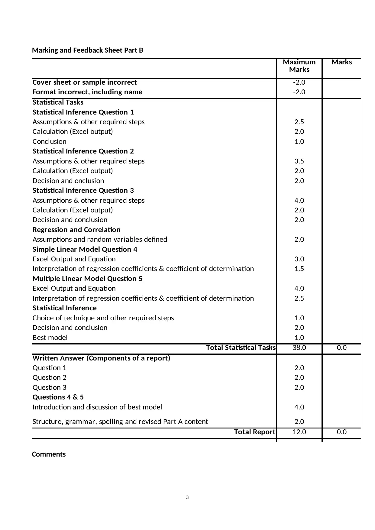
Marking and Feedback Sheet Part B
Marks
Cover sheet or sample incorrect -2.0
Format incorrect, including name -2.0
Statistical Tasks
Statistical Inference Question 1
Assumptions & other required steps 2.5
Calculation (Excel output) 2.0
Conclusion 1.0
Statistical Inference Question 2
Assumptions & other required steps 3.5
Calculation (Excel output) 2.0
Decision and onclusion 2.0
Statistical Inference Question 3
Assumptions & other required steps 4.0
Calculation (Excel output) 2.0
Decision and conclusion 2.0
Regression and Correlation
Assumptions and random variables defined 2.0
Simple Linear Model Question 4
Excel Output and Equation 3.0
Interpretation of regression coefficients & coefficient of determination 1.5
Multiple Linear Model Question 5
Excel Output and Equation 4.0
Interpretation of regression coefficients & coefficient of determination 2.5
Statistical Inference
Choice of technique and other required steps 1.0
Decision and conclusion 2.0
Best model 1.0
Total Statistical Tasks 38.0 0.0
Written Answer (Components of a report)
Question 1 2.0
Question 2 2.0
Question 3 2.0
Questions 4 & 5
Introduction and discussion of best model 4.0
Structure, grammar, spelling and revised Part A content 2.0
Total Report 12.0 0.0
Maximum
Marks
Comments
3

Dear Friend,
For estimating the population proportion of time for download speed to be at least
80% of the maximum speed, that is, 40 Mbps, the confidence interval has to be calculated.
Here, total number of population data will be considered, which is n = 120, for calculating
the population proportion.
Here, Internet speed data and time are random variables. Random variable,
generally denoted by X, represents a variable, which takes the possible values which are
numerical outcomes of a random event. Continuous and discrete are two types of random
variables, and in this case, internet speed is the continuous variable and Evening is the
discrete variable.
Estimation of the population proportion of time that the download speed is at least 40 Mbps
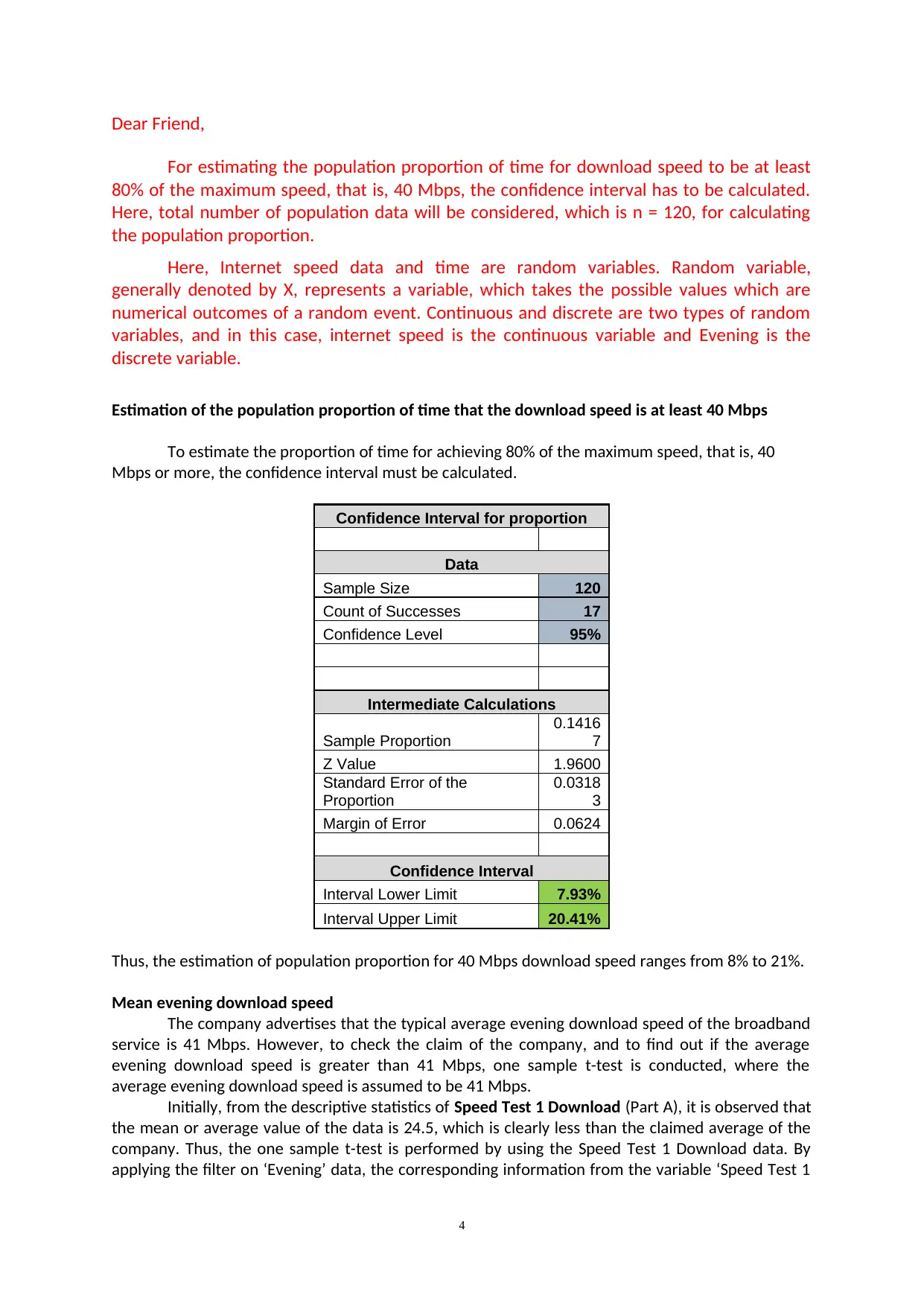
To estimate the proportion of time for achieving 80% of the maximum speed, that is, 40
Mbps or more, the confidence interval must be calculated.
Confidence Interval for proportion
Data
Sample Size 120
Count of Successes 17
Confidence Level 95%
Intermediate Calculations
Sample Proportion
0.1416
7
Z Value 1.9600
Standard Error of the
Proportion
0.0318
3
Margin of Error 0.0624
Confidence Interval
Interval Lower Limit 7.93%
Interval Upper Limit 20.41%
Thus, the estimation of population proportion for 40 Mbps download speed ranges from 8% to 21%.
Mean evening download speed
The company advertises that the typical average evening download speed of the broadband
service is 41 Mbps. However, to check the claim of the company, and to find out if the average
evening download speed is greater than 41 Mbps, one sample t-test is conducted, where the
average evening download speed is assumed to be 41 Mbps.
Initially, from the descriptive statistics of Speed Test 1 Download (Part A), it is observed that
the mean or average value of the data is 24.5, which is clearly less than the claimed average of the
company. Thus, the one sample t-test is performed by using the Speed Test 1 Download data. By
applying the filter on ‘Evening’ data, the corresponding information from the variable ‘Speed Test 1
4

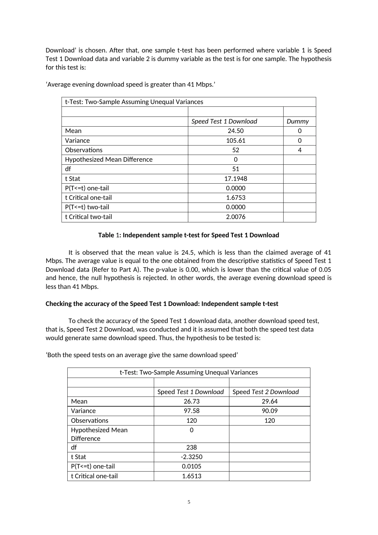
Download’ is chosen. After that, one sample t-test has been performed where variable 1 is Speed
Test 1 Download data and variable 2 is dummy variable as the test is for one sample. The hypothesis
for this test is:
‘Average evening download speed is greater than 41 Mbps.’
t-Test: Two-Sample Assuming Unequal Variances
Speed Test 1 Download Dummy
Mean 24.50 0
Variance 105.61 0
Observations 52 4
Hypothesized Mean Difference 0
df 51
t Stat 17.1948
P(T<=t) one-tail 0.0000
t Critical one-tail 1.6753
P(T<=t) two-tail 0.0000
t Critical two-tail 2.0076
Table 1: Independent sample t-test for Speed Test 1 Download
It is observed that the mean value is 24.5, which is less than the claimed average of 41
Mbps. The average value is equal to the one obtained from the descriptive statistics of Speed Test 1
Download data (Refer to Part A). The p-value is 0.00, which is lower than the critical value of 0.05
and hence, the null hypothesis is rejected. In other words, the average evening download speed is
less than 41 Mbps.
Checking the accuracy of the Speed Test 1 Download: Independent sample t-test
To check the accuracy of the Speed Test 1 download data, another download speed test,
that is, Speed Test 2 Download, was conducted and it is assumed that both the speed test data
would generate same download speed. Thus, the hypothesis to be tested is:
‘Both the speed tests on an average give the same download speed’
t-Test: Two-Sample Assuming Unequal Variances
Speed Test 1 Download Speed Test 2 Download
Mean 26.73 29.64
Variance 97.58 90.09
Observations 120 120
Hypothesized Mean
Difference
0
df 238
t Stat -2.3250
P(T<=t) one-tail 0.0105
t Critical one-tail 1.6513
5

P(T<=t) two-tail 0.0209
t Critical two-tail 1.9700
Table 2: Independent sample t-test for Speed Test 1 Download and Speed Test 2 Download
It is found that the average value or mean for Speed Test 1 and Speed Test 2 are different,
26.73 and 29.64 respectively. The t-stat value (-2.325) is less than the –t critical two-tail (-1.97) and
hence, the null hypothesis is rejected. Therefore, it is proved that the two speed tests do not
generate the same average speed.
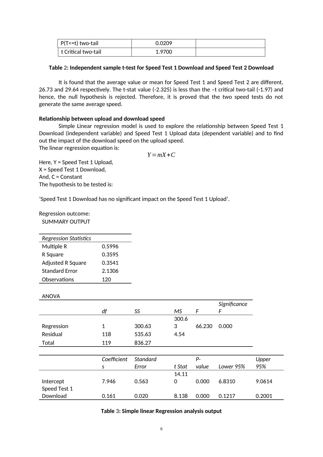
Relationship between upload and download speed
Simple Linear regression model is used to explore the relationship between Speed Test 1
Download (independent variable) and Speed Test 1 Upload data (dependent variable) and to find
out the impact of the download speed on the upload speed.
The linear regression equation is:
Y =mX +C
Here, Y = Speed Test 1 Upload,
X = Speed Test 1 Download,
And, C = Constant
The hypothesis to be tested is:
‘Speed Test 1 Download has no significant impact on the Speed Test 1 Upload’.
Regression outcome:
SUMMARY OUTPUT
Regression Statistics
Multiple R 0.5996
R Square 0.3595
Adjusted R Square 0.3541
Standard Error 2.1306
Observations 120
ANOVA
df SS MS F
Significance
F
Regression 1 300.63
300.6
3 66.230 0.000
Residual 118 535.63 4.54
Total 119 836.27
Coefficient
s
Standard
Error t Stat
P-
value Lower 95%
Upper
95%
Intercept 7.946 0.563
14.11
0 0.000 6.8310 9.0614
Speed Test 1
Download 0.161 0.020 8.138 0.000 0.1217 0.2001
Table 3: Simple linear Regression analysis output
6

5.00 10.00 15.00 20.00 25.00 30.00 35.00 40.00 45.00 50.00
0.00
2.00
4.00
6.00
8.00
10.00
12.00
14.00
16.00
18.00
f(x) = 0.160899416432325 x + 7.9462045908683
R² = 0.359495525927541
Speed Test 1 Upload
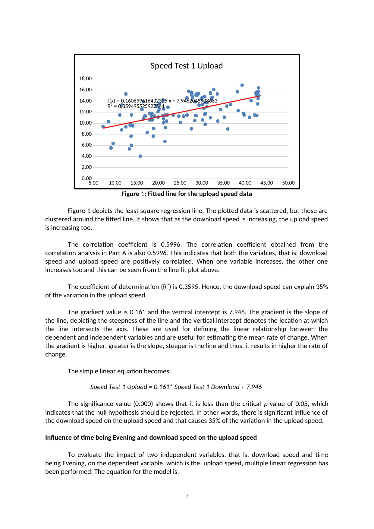
Figure 1: Fitted line for the upload speed data
Figure 1 depicts the least square regression line. The plotted data is scattered, but those are
clustered around the fitted line. It shows that as the download speed is increasing, the upload speed
is increasing too.
The correlation coefficient is 0.5996. The correlation coefficient obtained from the
correlation analysis in Part A is also 0.5996. This indicates that both the variables, that is, download
speed and upload speed are positively correlated. When one variable increases, the other one
increases too and this can be seen from the line fit plot above.
The coefficient of determination (R2) is 0.3595. Hence, the download speed can explain 35%
of the variation in the upload speed.
The gradient value is 0.161 and the vertical intercept is 7.946. The gradient is the slope of
the line, depicting the steepness of the line and the vertical intercept denotes the location at which
the line intersects the axis. These are used for defining the linear relationship between the
dependent and independent variables and are useful for estimating the mean rate of change. When
the gradient is higher, greater is the slope, steeper is the line and thus, it results in higher the rate of
change.
The simple linear equation becomes:
Speed Test 1 Upload = 0.161* Speed Test 1 Download + 7.946
The significance value (0.000) shows that it is less than the critical p-value of 0.05, which
indicates that the null hypothesis should be rejected. In other words, there is significant influence of
the download speed on the upload speed and that causes 35% of the variation in the upload speed.
Influence of time being Evening and download speed on the upload speed
To evaluate the impact of two independent variables, that is, download speed and time
being Evening, on the dependent variable, which is the, upload speed, multiple linear regression has
been performed. The equation for the model is:
7

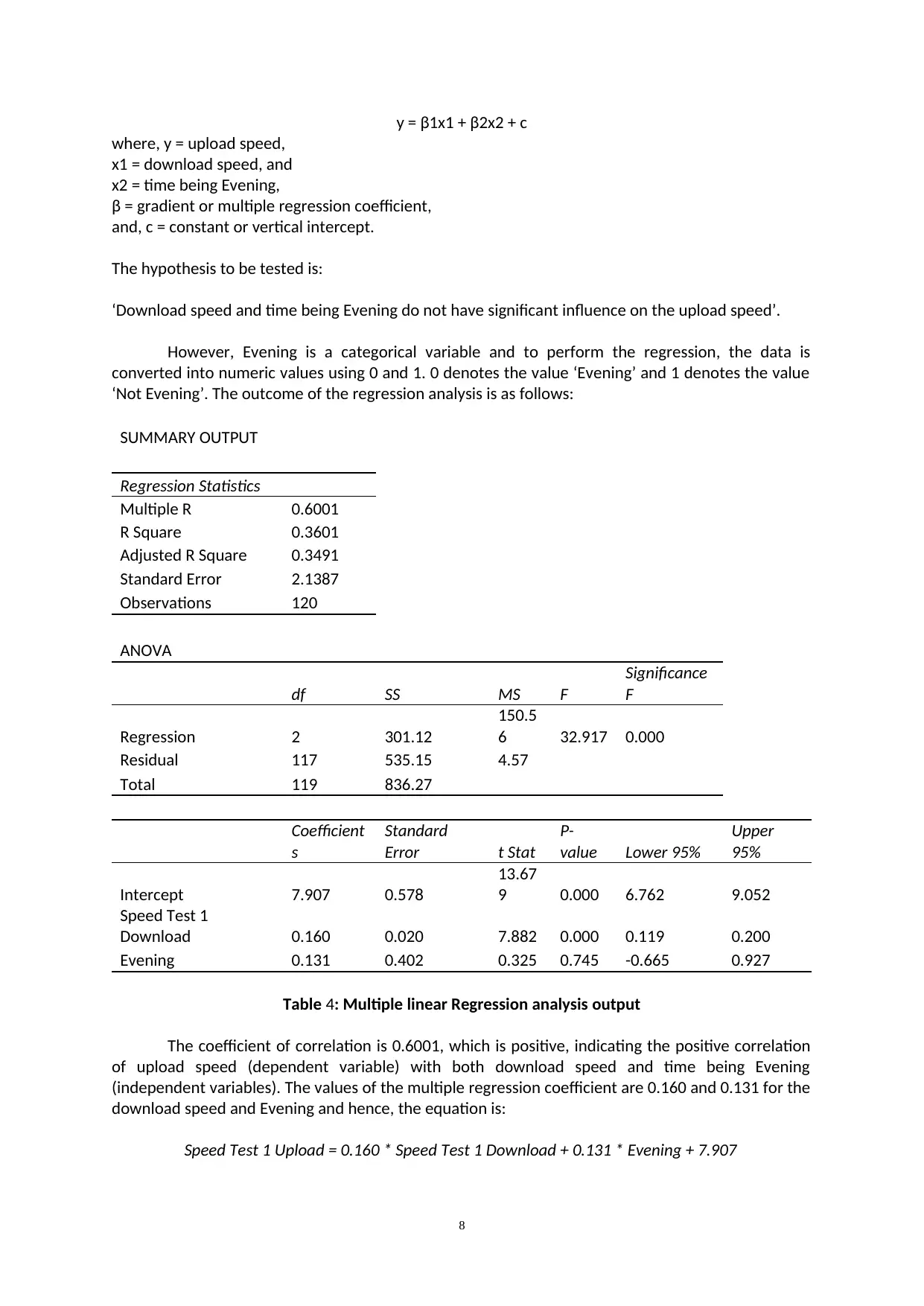
y = β1x1 + β2x2 + c
where, y = upload speed,
x1 = download speed, and
x2 = time being Evening,
β = gradient or multiple regression coefficient,
and, c = constant or vertical intercept.
The hypothesis to be tested is:
‘Download speed and time being Evening do not have significant influence on the upload speed’.
However, Evening is a categorical variable and to perform the regression, the data is
converted into numeric values using 0 and 1. 0 denotes the value ‘Evening’ and 1 denotes the value
‘Not Evening’. The outcome of the regression analysis is as follows:
SUMMARY OUTPUT
Regression Statistics
Multiple R 0.6001
R Square 0.3601
Adjusted R Square 0.3491
Standard Error 2.1387
Observations 120
ANOVA
df SS MS F
Significance
F
Regression 2 301.12
150.5
6 32.917 0.000
Residual 117 535.15 4.57
Total 119 836.27
Coefficient
s
Standard
Error t Stat
P-
value Lower 95%
Upper
95%
Intercept 7.907 0.578
13.67
9 0.000 6.762 9.052
Speed Test 1
Download 0.160 0.020 7.882 0.000 0.119 0.200
Evening 0.131 0.402 0.325 0.745 -0.665 0.927
Table 4: Multiple linear Regression analysis output
The coefficient of correlation is 0.6001, which is positive, indicating the positive correlation
of upload speed (dependent variable) with both download speed and time being Evening
(independent variables). The values of the multiple regression coefficient are 0.160 and 0.131 for the
download speed and Evening and hence, the equation is:
Speed Test 1 Upload = 0.160 * Speed Test 1 Download + 0.131 * Evening + 7.907
8

When time is Evening, the regression equation is:
Speed Test 1 Upload = 0.160 * Speed Test 1 Download + 0.131 * 0 + 7.907
= 0.160 * Speed Test 1 Download + 7.907
When time is Not Evening, the regression equation is:
Speed Test 1 Upload = 0.160 * Speed Test 1 Download + 0.131 * 1 + 7.907
= 0.160 * Speed Test 1 Download + 0.131 + 7.907
= 0.160 * Speed Test 1 Download + 8.038
Thus, with increase in both the variables, upload speed increases. However, as time takes 0
and 1 values for Evening and Not Evening respectively, the value of the vertical intercept changes,
hence, it can be said that the upload speed is higher during Not Evening than in case of Evening.
The coefficient of determination (R2) is 0.3601, indicating that the variables, download speed
and time being Evening, can explain 36% of the variations in the upload speed.
It is seen that in simple linear model, the coefficient of determination explains 35% of the
variations in the upload speed, while that is 36% in case of multiple linear regression. Individually,
download speed has larger impact on the upload speed as the p-value is 0.00, which is lower than
0.05, while the p-value of ‘Evening’ is 0.74, which is much larger than 0.05. Thus, Evening does not
contribute much to the model or variations in the upload speed. Thus, the multiple linear regression
model is more suitable or best fit to explain the variations in the upload speed. Moreover, the
significance value is found to be less than 0.05, which also implies that the null hypothesis is
rejected. Thus, the download speed and Evening both have influence on the upload speed.
Sincerely,
[Name of the student].
9

Bibliography
Carlson, K.A. and Winquist, J.R., 2016. An introduction to statistics: An active learning approach. Sage
Publications.
Heumann, C. and Schomaker, M., 2016. Introduction to statistics and data analysis. Springer
International Publishing Switzerland.
Holcomb, Z.C., 2016. Fundamentals of descriptive statistics. Routledge.
Moore, D.S., McCabe, G.P., Alwan, L.C., Craig, B.A. and Duckworth, W.M., 2016. The practice of
statistics for business and economics. WH Freeman.
10