Week 1 Project: Statistical Analysis and Hypothesis Testing Report

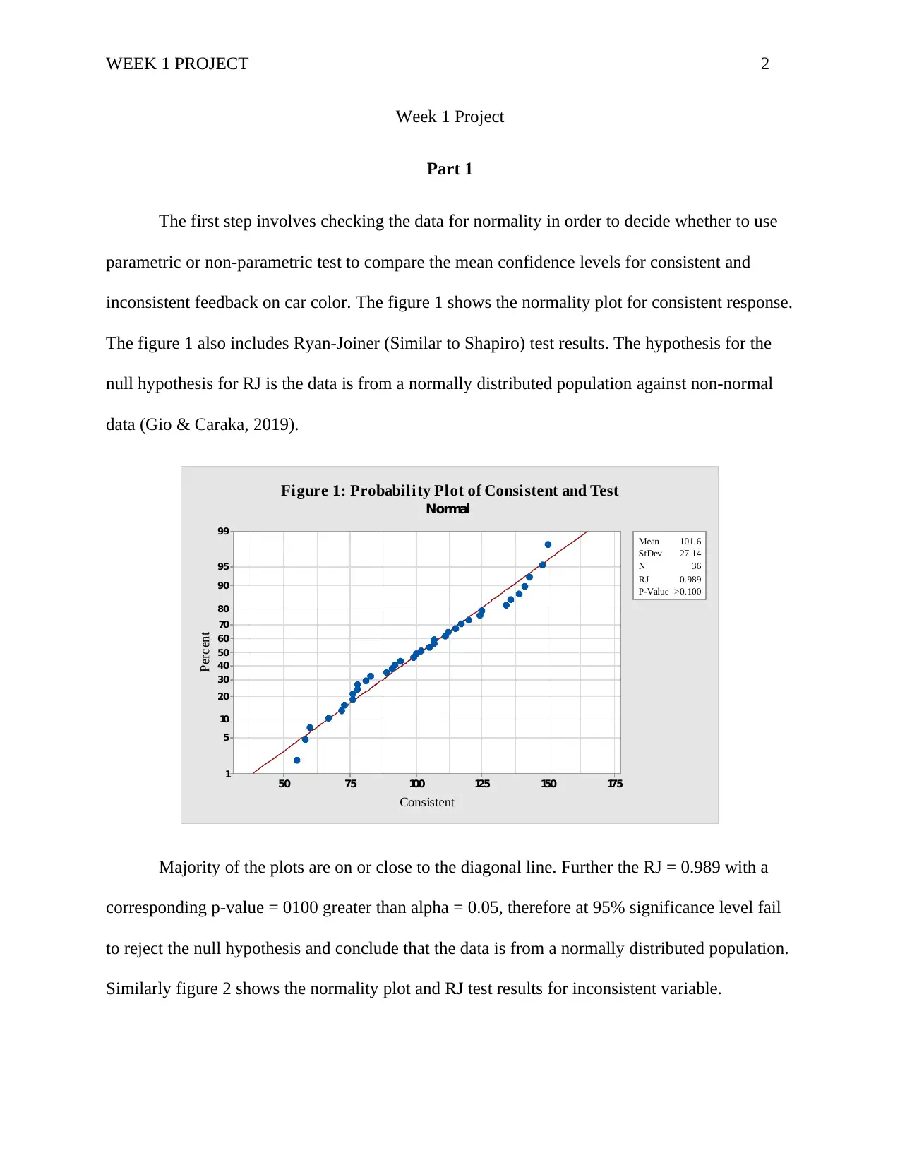
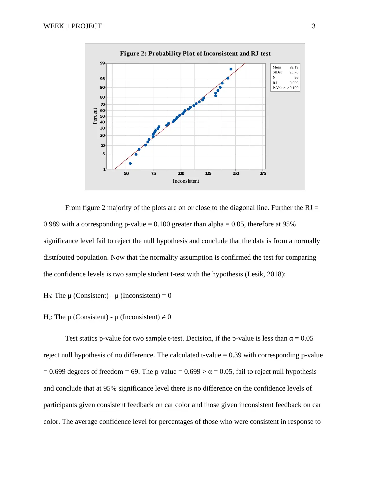
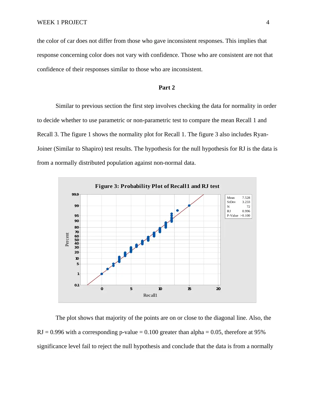
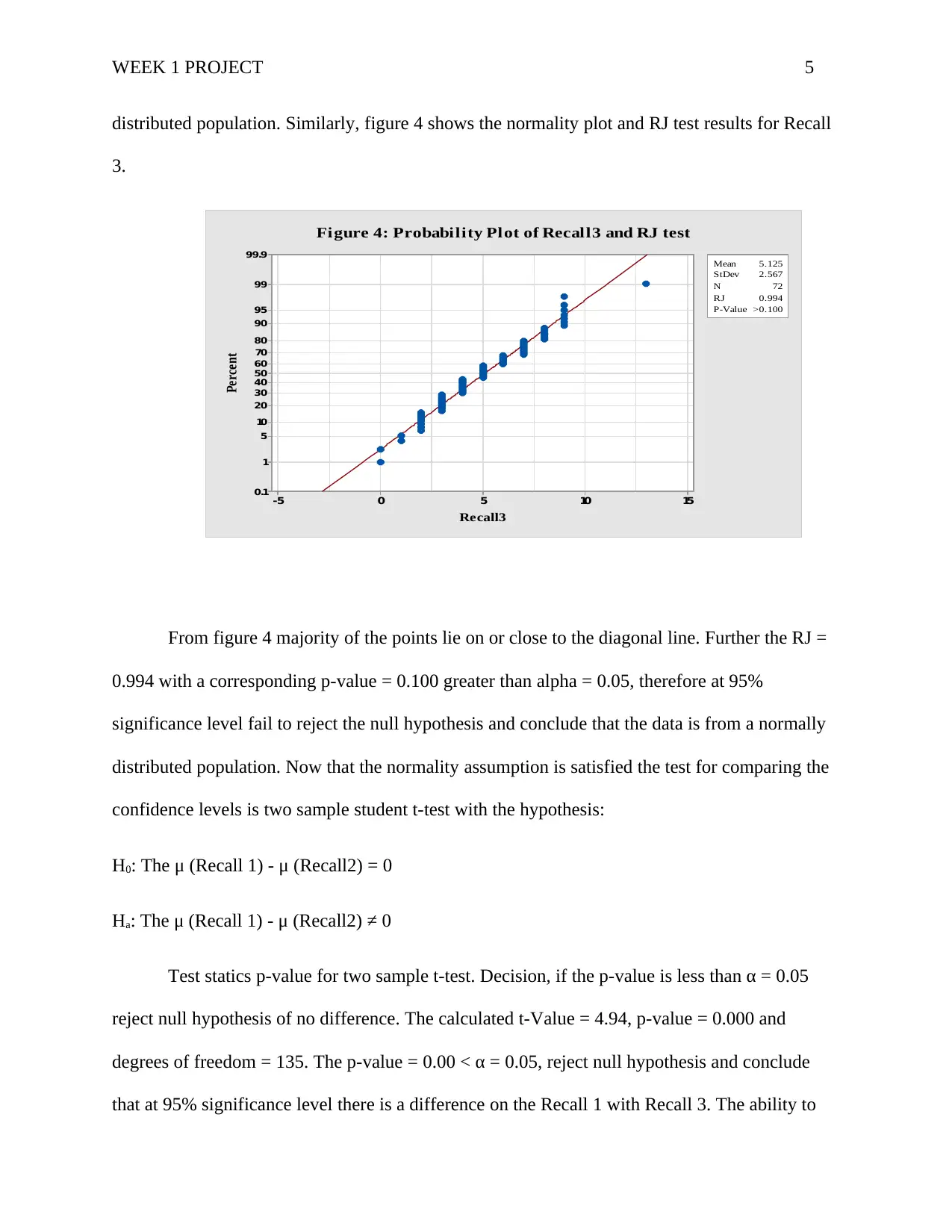
This project presents a statistical analysis of two datasets. The analysis begins by checking for data normality using probability plots and the Ryan-Joiner test. The project then employs two-sample student t-tests to compare confidence levels in the first dataset, concluding that there is no significant difference between consistent and inconsistent feedback on car color. The second part of the project similarly tests for normality and uses t-tests to compare recall abilities at different times, finding a significant difference between the first and third recalls, indicating a decrease in recall ability over time. The analysis includes statistical values such as t-values, p-values, and degrees of freedom, and interprets these values to draw conclusions about the data. The project is supported by references to relevant statistical resources.

Running head: WEEK 1 PROJECT 1
Week 1 Project
Name
Institution

WEEK 1 PROJECT 2
Week 1 Project
Part 1
The first step involves checking the data for normality in order to decide whether to use
parametric or non-parametric test to compare the mean confidence levels for consistent and
inconsistent feedback on car color. The figure 1 shows the normality plot for consistent response.
The figure 1 also includes Ryan-Joiner (Similar to Shapiro) test results. The hypothesis for the
null hypothesis for RJ is the data is from a normally distributed population against non-normal
data (Gio & Caraka, 2019).
1751501251007550
99
95
90
80
70
60
50
40
30
20
10
5
1
Mean 101.6
StDev 27.14
N 36
RJ 0.989
P-Value >0.100
Consistent
Percent
Figure 1: Probability Plot of Consistent and Test
Normal
Majority of the plots are on or close to the diagonal line. Further the RJ = 0.989 with a
corresponding p-value = 0100 greater than alpha = 0.05, therefore at 95% significance level fail
to reject the null hypothesis and conclude that the data is from a normally distributed population.
Similarly figure 2 shows the normality plot and RJ test results for inconsistent variable.

WEEK 1 PROJECT 3
1751501251007550
99
95
90
80
70
60
50
40
30
20
10
5
1
Mean 99.19
StDev 25.70
N 36
RJ 0.989
P-Value >0.100
Inconsistent
Percent
Figure 2: Probability Plot of Inconsistent and RJ test
From figure 2 majority of the plots are on or close to the diagonal line. Further the RJ =
0.989 with a corresponding p-value = 0.100 greater than alpha = 0.05, therefore at 95%
significance level fail to reject the null hypothesis and conclude that the data is from a normally
distributed population. Now that the normality assumption is confirmed the test for comparing
the confidence levels is two sample student t-test with the hypothesis (Lesik, 2018):
H0: The μ (Consistent) - μ (Inconsistent) = 0
Ha: The μ (Consistent) - μ (Inconsistent) ≠ 0
Test statics p-value for two sample t-test. Decision, if the p-value is less than α = 0.05
reject null hypothesis of no difference. The calculated t-value = 0.39 with corresponding p-value
= 0.699 degrees of freedom = 69. The p-value = 0.699 > α = 0.05, fail to reject null hypothesis
and conclude that at 95% significance level there is no difference on the confidence levels of
participants given consistent feedback on car color and those given inconsistent feedback on car
color. The average confidence level for percentages of those who were consistent in response to

WEEK 1 PROJECT 4
the color of car does not differ from those who gave inconsistent responses. This implies that
response concerning color does not vary with confidence. Those who are consistent are not that
confidence of their responses similar to those who are inconsistent.
Part 2
Similar to previous section the first step involves checking the data for normality in order
to decide whether to use parametric or non-parametric test to compare the mean Recall 1 and
Recall 3. The figure 1 shows the normality plot for Recall 1. The figure 3 also includes Ryan-
Joiner (Similar to Shapiro) test results. The hypothesis for the null hypothesis for RJ is the data is
from a normally distributed population against non-normal data.
20151050
99.9
99
95
90
80
70
60
50
40
30
20
10
5
1
0.1
Mean 7.528
StDev 3.233
N 72
RJ 0.996
P-Value >0.100
Recall1
Percent
Figure 3: Probability Plot of Recall1 and RJ test
The plot shows that majority of the points are on or close to the diagonal line. Also, the
RJ = 0.996 with a corresponding p-value = 0.100 greater than alpha = 0.05, therefore at 95%
significance level fail to reject the null hypothesis and conclude that the data is from a normally

WEEK 1 PROJECT 5
distributed population. Similarly, figure 4 shows the normality plot and RJ test results for Recall
3.
151050-5
99.9
99
95
90
80
70
60
50
40
30
20
10
5
1
0.1
Mean 5.125
StDev 2.567
N 72
RJ 0.994
P-Value >0.100
Recall3
Percent
Figure 4: Probability Plot of Recall3 and RJ test
From figure 4 majority of the points lie on or close to the diagonal line. Further the RJ =
0.994 with a corresponding p-value = 0.100 greater than alpha = 0.05, therefore at 95%
significance level fail to reject the null hypothesis and conclude that the data is from a normally
distributed population. Now that the normality assumption is satisfied the test for comparing the
confidence levels is two sample student t-test with the hypothesis:
H0: The μ (Recall 1) - μ (Recall2) = 0
Ha: The μ (Recall 1) - μ (Recall2) ≠ 0
Test statics p-value for two sample t-test. Decision, if the p-value is less than α = 0.05
reject null hypothesis of no difference. The calculated t-Value = 4.94, p-value = 0.000 and
degrees of freedom = 135. The p-value = 0.00 < α = 0.05, reject null hypothesis and conclude
that at 95% significance level there is a difference on the Recall 1 with Recall 3. The ability to

WEEK 1 PROJECT 6
recall for the first time is different to the ability to recall for the third time. The average correct
recalling for first time is 7.528 while for third time is 5.125. Thus, the average recalling ability
decreases with the number of recalls.

WEEK 1 PROJECT 7
References
Gio, P. U., & Caraka, R. E. (2019). Normality Assumption Test Using STATCAL (R), SPSS,
Eviews and Minitab.
Lesik, S. A. (2018). Applied Statistical Inference with MINITAB®. Chapman and Hall/CRC.