University R Programming and Statistical Analysis Homework Solutions

The assignment solutions presented involve using R programming for statistical analysis. The document includes code and output for several exercises, such as analyzing the relationship between Calcium and ProteinProp, Time and Elevation, and exploring ANOVA. It covers tasks like fitting linear models, generating plots, calculating correlations, and interpreting statistical summaries. The code demonstrates data import, model fitting, and visualization techniques. The document also includes solutions for exercises involving multiple linear regression and analysis of variance (ANOVA) to determine relationships between different variables. The student has used R statistical software to address various problems related to data analysis, model building, and interpretation of results, including the use of multiple datasets.

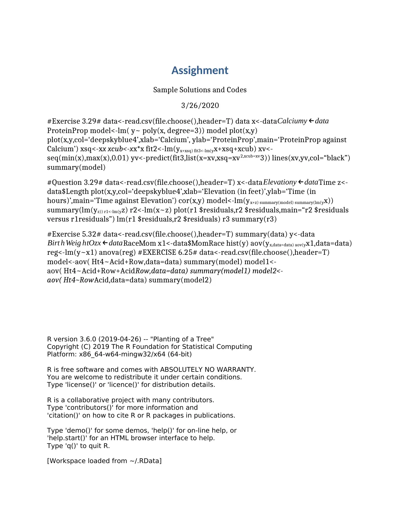
Assighment
Sample Solutions and Codes
3/26/2020
#Exercise 3.29# data<-read.csv(file.choose(),header=T) data x<-data Calciumy ←data
ProteinProp model<-lm( y~ poly(x, degree=3)) model plot(x,y)
plot(x,y,col=‘deepskyblue4’,xlab=‘Calcium’, ylab=‘ProteinProp’,main=‘ProteinProp against
Calcium’) xsq<-xx xcub<-xx*x fit2<-lm(yx+xsq) fit3<-lm(yx+xsq+xcub) xv<-
seq(min(x),max(x),0.01) yv<-predict(fit3,list(x=xv,xsq=xv2,xcub=xv3)) lines(xv,yv,col=“black”)
summary(model)
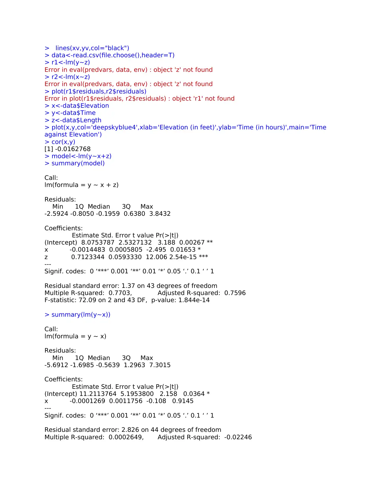
#Question 3.29# data<-read.csv(file.choose(),header=T) x<-dataElevationy ←dataTime z<-
data$Length plot(x,y,col=‘deepskyblue4’,xlab=‘Elevation (in feet)’,ylab=‘Time (in
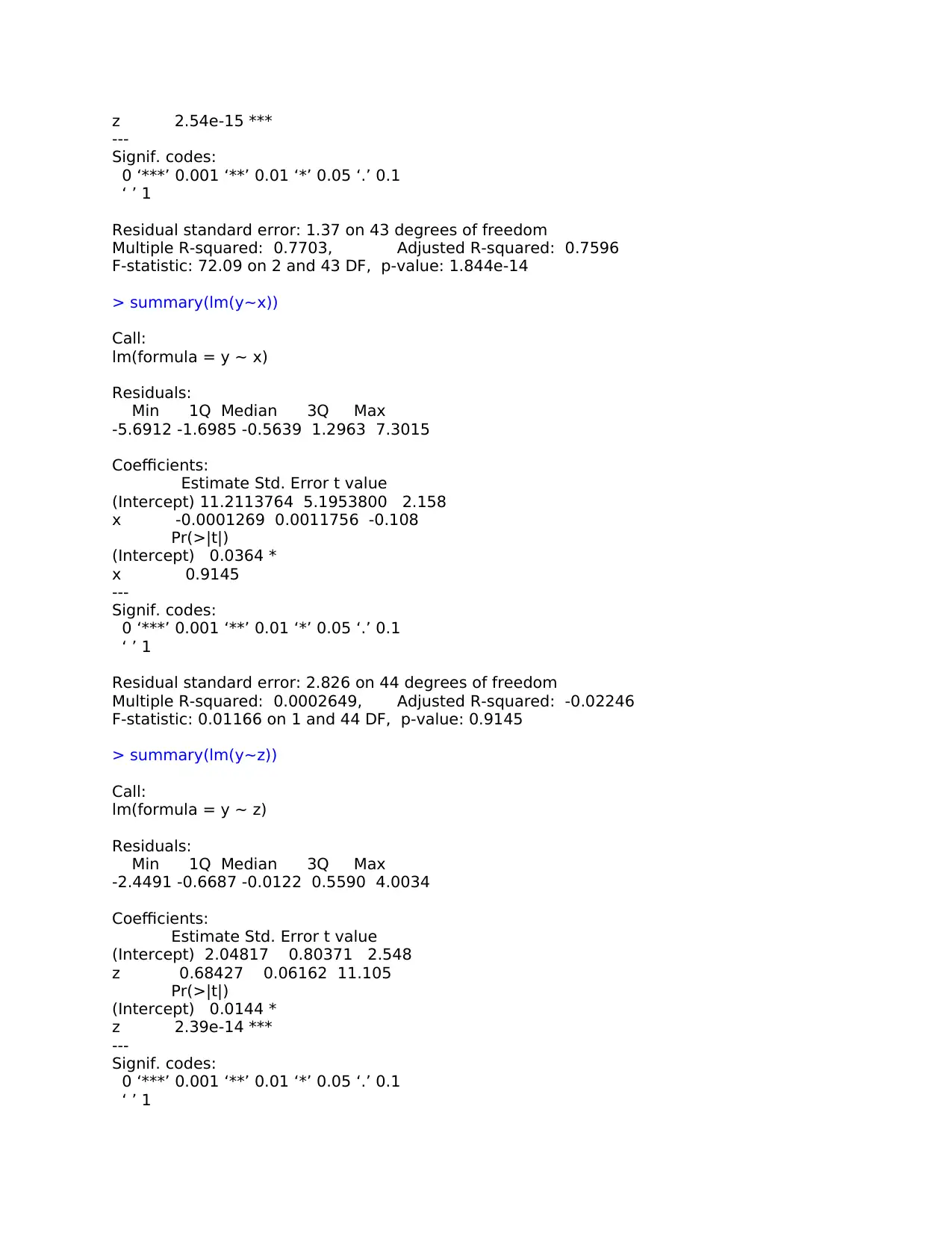
hours)’,main=‘Time against Elevation’) cor(x,y) model<-lm(yx+z) summary(model) summary(lm(yx))
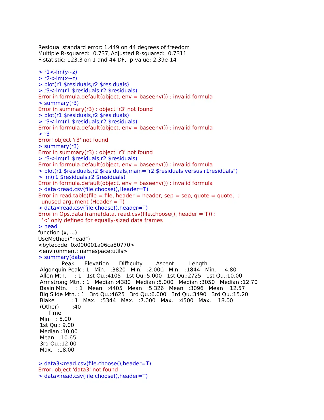
summary(lm(yz)) r1<-lm(yz) r2<-lm(x~z) plot(r1 $residuals,r2 $residuals,main=“r2 $residuals
versus r1residuals”) lm(r1 $residuals,r2 $residuals) r3 summary(r3)
#Exercise 5.32# data<-read.csv(file.choose(),header=T) summary(data) y<-data
Birt h Weig htOzx ←dataRaceMom x1<-data$MomRace hist(y) aov(yx,data=data) aov(yx1,data=data)
reg<-lm(y~x1) anova(reg) #EXERCISE 6.25# data<-read.csv(file.choose(),header=T)
model<-aov( Ht4~Acid+Row,data=data) summary(model) model1<-
aov( Ht4~Acid+Row+AcidRow,data=data) summary(model1) model2<-
aov( Ht4~RowAcid,data=data) summary(model2)
R version 3.6.0 (2019-04-26) -- "Planting of a Tree"
Copyright (C) 2019 The R Foundation for Statistical Computing
Platform: x86_64-w64-mingw32/x64 (64-bit)
R is free software and comes with ABSOLUTELY NO WARRANTY.
You are welcome to redistribute it under certain conditions.
Type 'license()' or 'licence()' for distribution details.
R is a collaborative project with many contributors.
Type 'contributors()' for more information and
'citation()' on how to cite R or R packages in publications.
Type 'demo()' for some demos, 'help()' for on-line help, or
'help.start()' for an HTML browser interface to help.
Type 'q()' to quit R.
[Workspace loaded from ~/.RData]

> data<-read.csv(file.choose(),header=T)
> data
Calcium ProteinProp
1 -10.145390 0.1451642
2 -9.977984 0.2237115
3 -9.351250 0.2198288
4 -9.101001 0.3342694
5 -9.013766 0.3785262
6 -8.940437 0.4093691
7 -8.578232 0.5074450
8 -8.370183 0.5716413
9 -8.289037 0.6421870
10 -7.959793 0.8072800
11 -7.592269 0.9300252
12 -7.238448 0.9014096
13 -7.038626 0.9503276
14 -6.330776 0.9573205
15 -6.167236 0.9851045
16 -5.556894 0.9694070
17 -5.321209 0.9992852
18 -4.813609 1.0000000
19 -10.145390 0.1882841
20 -9.977984 0.2268408
21 -9.351250 0.2998251
22 -9.101001 0.3517163
23 -9.013766 0.4139161
24 -8.940437 0.4374755
25 -8.578232 0.5263771
26 -8.370183 0.6197400
27 -8.289037 0.6709965
28 -7.959793 0.8444435
29 -7.592269 0.9298122
30 -7.238448 0.9798032
31 -7.038626 0.9742129
32 -6.330776 0.9742309
33 -6.167236 0.9875247
34 -5.556894 0.9982300
35 -5.321209 1.0000000
36 -4.813609 0.9957145
37 -10.721933 0.2647664
38 -10.445753 0.3369681
39 -9.689732 0.4011040
40 -9.047837 0.3971727
41 -8.791559 0.5356422
42 -8.448916 0.6486877
43 -8.088203 0.6680274
44 -7.851397 0.8055475
45 -7.658565 0.8586845
46 -7.482276 0.8798047
47 -7.306449 1.0000000
48 -7.115545 0.9771862
49 -6.884057 0.9651696
50 -6.539854 0.9645220
51 -5.865186 0.9858963

> x<-data$Calcium
> y<-data$ProteinProp
> model<-lm( y~ poly(x, degree=3))
> model
Call:
lm(formula = y ~ poly(x, degree = 3))
Coefficients:
(Intercept) poly(x, degree = 3)1 poly(x, degree = 3)2 poly(x, degree = 3)3
0.6871 1.8962 -0.4988 -0.4673
> plot(x,y)
> plot(x,y,col='deepskyblue4',xlab='Calcium', ylab='ProteinProp',main='ProteinProp
against Calcium ')
> xsq<-x*x
> xcub<-x*x*x
> fit2<-lm(y~x+xsq)
> fit3<-lm(y~x+xsq+xcub)
> xv<-seq(min(x),max(x),0.01)
> yv<-predict(fit3,list(x=xv,xsq=xv^2,xcub=xv^3))
> lines(xv,yv,col="black")
> lines(x,col='green',lwd=3)
> lines(model,lwd=3,col='purple')
Error in xy.coords(x, y) :
'x' is a list, but does not have components 'x' and 'y'
> lines(y,col='purple',lwd=3)
> lines(x,y,predict(model),col='red')
Error in plot.xy(xy.coords(x, y), type = type, ...) : invalid plot type
> summary(model)
Call:
lm(formula = y ~ poly(x, degree = 3))
Residuals:
Min 1Q Median 3Q Max
-0.14031 -0.05528 -0.01859 0.05267 0.13583
Coefficients:
Estimate Std. Error t value Pr(>|t|)
(Intercept) 0.68707 0.00994 69.120 < 2e-16 ***
poly(x, degree = 3)1 1.89623 0.07099 26.712 < 2e-16 ***
poly(x, degree = 3)2 -0.49882 0.07099 -7.027 7.44e-09 ***
poly(x, degree = 3)3 -0.46729 0.07099 -6.583 3.51e-08 ***
---
Signif. codes: 0 ‘***’ 0.001 ‘**’ 0.01 ‘*’ 0.05 ‘.’ 0.1 ‘ ’ 1
Residual standard error: 0.07099 on 47 degrees of freedom
Multiple R-squared: 0.9449, Adjusted R-squared: 0.9414
F-statistic: 268.8 on 3 and 47 DF, p-value: < 2.2e-16
> plot(x,y,col='deepskyblue4',xlab='Calcium', ylab='ProteinProp',main='ProteinProp against
Calcium ')
> xv<-seq(min(x),max(x),0.01)
> yv<-predict(fit3,list(x=xv,xsq=xv^2,xcub=xv^3))

> lines(xv,yv,col="black")
> data<-read.csv(file.choose(),header=T)
> r1<-lm(y~z)
Error in eval(predvars, data, env) : object 'z' not found
> r2<-lm(x~z)
Error in eval(predvars, data, env) : object 'z' not found
> plot(r1$residuals,r2$residuals)
Error in plot(r1$residuals, r2$residuals) : object 'r1' not found
> x<-data$Elevation
> y<-data$Time
> z<-data$Length
> plot(x,y,col='deepskyblue4',xlab='Elevation (in feet)',ylab='Time (in hours)',main='Time
against Elevation')
> cor(x,y)
[1] -0.0162768
> model<-lm(y~x+z)
> summary(model)
Call:
lm(formula = y ~ x + z)
Residuals:
Min 1Q Median 3Q Max
-2.5924 -0.8050 -0.1959 0.6380 3.8432
Coefficients:
Estimate Std. Error t value Pr(>|t|)
(Intercept) 8.0753787 2.5327132 3.188 0.00267 **
x -0.0014483 0.0005805 -2.495 0.01653 *
z 0.7123344 0.0593330 12.006 2.54e-15 ***
---
Signif. codes: 0 ‘***’ 0.001 ‘**’ 0.01 ‘*’ 0.05 ‘.’ 0.1 ‘ ’ 1
Residual standard error: 1.37 on 43 degrees of freedom
Multiple R-squared: 0.7703, Adjusted R-squared: 0.7596
F-statistic: 72.09 on 2 and 43 DF, p-value: 1.844e-14
> summary(lm(y~x))
Call:
lm(formula = y ~ x)
Residuals:
Min 1Q Median 3Q Max
-5.6912 -1.6985 -0.5639 1.2963 7.3015
Coefficients:
Estimate Std. Error t value Pr(>|t|)
(Intercept) 11.2113764 5.1953800 2.158 0.0364 *
x -0.0001269 0.0011756 -0.108 0.9145
---
Signif. codes: 0 ‘***’ 0.001 ‘**’ 0.01 ‘*’ 0.05 ‘.’ 0.1 ‘ ’ 1
Residual standard error: 2.826 on 44 degrees of freedom
Multiple R-squared: 0.0002649, Adjusted R-squared: -0.02246

F-statistic: 0.01166 on 1 and 44 DF, p-value: 0.9145
> summary(lm(y~z))
Call:
lm(formula = y ~ z)
Residuals:
Min 1Q Median 3Q Max
-2.4491 -0.6687 -0.0122 0.5590 4.0034
Coefficients:
Estimate Std. Error t value Pr(>|t|)
(Intercept) 2.04817 0.80371 2.548 0.0144 *
z 0.68427 0.06162 11.105 2.39e-14 ***
---
Signif. codes: 0 ‘***’ 0.001 ‘**’ 0.01 ‘*’ 0.05 ‘.’ 0.1 ‘ ’ 1
Residual standard error: 1.449 on 44 degrees of freedom
Multiple R-squared: 0.737, Adjusted R-squared: 0.7311
F-statistic: 123.3 on 1 and 44 DF, p-value: 2.39e-14
> r1<-lm(y~z)
> r2<-lm(x~z)
> plot(r1$residuals,r2$residuals)
> plot(r1 $residuals,r2 $residuals)
> r3<-lm(r1 $residuals,r2 $residuals)
Error in formula.default(object, env = baseenv()) : invalid formula
> summary(r3)
Error in summary(r3) : object 'r3' not found
> x<-data$Elevation
> y<-data$Time
> z<-data$Length
> plot(x,y,col='deepskyblue4',xlab='Elevation (in feet)',ylab='Time (in hours)',main='Time
against Elevation')
> cor(x,y)
[1] -0.0162768
> model<-lm(y~x+z)
> summary(model)
Call:
lm(formula = y ~ x + z)
Residuals:
Min 1Q Median 3Q Max
-2.5924 -0.8050 -0.1959 0.6380 3.8432
Coefficients:
Estimate Std. Error t value
(Intercept) 8.0753787 2.5327132 3.188
x -0.0014483 0.0005805 -2.495
z 0.7123344 0.0593330 12.006
Pr(>|t|)
(Intercept) 0.00267 **
x 0.01653 *

z 2.54e-15 ***
---
Signif. codes:
0 ‘***’ 0.001 ‘**’ 0.01 ‘*’ 0.05 ‘.’ 0.1
‘ ’ 1
Residual standard error: 1.37 on 43 degrees of freedom
Multiple R-squared: 0.7703, Adjusted R-squared: 0.7596
F-statistic: 72.09 on 2 and 43 DF, p-value: 1.844e-14
> summary(lm(y~x))
Call:
lm(formula = y ~ x)
Residuals:
Min 1Q Median 3Q Max
-5.6912 -1.6985 -0.5639 1.2963 7.3015
Coefficients:
Estimate Std. Error t value
(Intercept) 11.2113764 5.1953800 2.158
x -0.0001269 0.0011756 -0.108
Pr(>|t|)
(Intercept) 0.0364 *
x 0.9145
---
Signif. codes:
0 ‘***’ 0.001 ‘**’ 0.01 ‘*’ 0.05 ‘.’ 0.1
‘ ’ 1
Residual standard error: 2.826 on 44 degrees of freedom
Multiple R-squared: 0.0002649, Adjusted R-squared: -0.02246
F-statistic: 0.01166 on 1 and 44 DF, p-value: 0.9145
> summary(lm(y~z))
Call:
lm(formula = y ~ z)
Residuals:
Min 1Q Median 3Q Max
-2.4491 -0.6687 -0.0122 0.5590 4.0034
Coefficients:
Estimate Std. Error t value
(Intercept) 2.04817 0.80371 2.548
z 0.68427 0.06162 11.105
Pr(>|t|)
(Intercept) 0.0144 *
z 2.39e-14 ***
---
Signif. codes:
0 ‘***’ 0.001 ‘**’ 0.01 ‘*’ 0.05 ‘.’ 0.1
‘ ’ 1

Residual standard error: 1.449 on 44 degrees of freedom
Multiple R-squared: 0.737, Adjusted R-squared: 0.7311
F-statistic: 123.3 on 1 and 44 DF, p-value: 2.39e-14
> r1<-lm(y~z)
> r2<-lm(x~z)
> plot(r1 $residuals,r2 $residuals)
> r3<-lm(r1 $residuals,r2 $residuals)
Error in formula.default(object, env = baseenv()) : invalid formula
> summary(r3)
Error in summary(r3) : object 'r3' not found
> plot(r1 $residuals,r2 $residuals)
> r3<-lm(r1 $residuals,r2 $residuals)
Error in formula.default(object, env = baseenv()) : invalid formula
> r3
Error: object 'r3' not found
> summary(r3)
Error in summary(r3) : object 'r3' not found
> r3<-lm(r1 $residuals,r2 $residuals)
Error in formula.default(object, env = baseenv()) : invalid formula
> plot(r1 $residuals,r2 $residuals,main="r2 $residuals versus r1residuals")
> lm(r1 $residuals,r2 $residuals)
Error in formula.default(object, env = baseenv()) : invalid formula
> data<read.csv(file.choose(),Header=T)
Error in read.table(file = file, header = header, sep = sep, quote = quote, :
unused argument (Header = T)
> data<read.csv(file.choose(),header=T)
Error in Ops.data.frame(data, read.csv(file.choose(), header = T)) :
‘<’ only defined for equally-sized data frames
> head
function (x, ...)
UseMethod("head")
<bytecode: 0x000001a06ca80770>
<environment: namespace:utils>
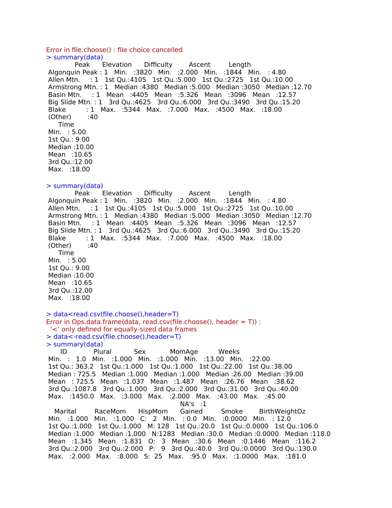
> summary(data)
Peak Elevation Difficulty Ascent Length
Algonquin Peak : 1 Min. :3820 Min. :2.000 Min. :1844 Min. : 4.80
Allen Mtn. : 1 1st Qu.:4105 1st Qu.:5.000 1st Qu.:2725 1st Qu.:10.00
Armstrong Mtn. : 1 Median :4380 Median :5.000 Median :3050 Median :12.70
Basin Mtn. : 1 Mean :4405 Mean :5.326 Mean :3096 Mean :12.57
Big Slide Mtn. : 1 3rd Qu.:4625 3rd Qu.:6.000 3rd Qu.:3490 3rd Qu.:15.20
Blake : 1 Max. :5344 Max. :7.000 Max. :4500 Max. :18.00
(Other) :40
Time
Min. : 5.00
1st Qu.: 9.00
Median :10.00
Mean :10.65
3rd Qu.:12.00
Max. :18.00
> data3<read.csv(file.choose(),header=T)
Error: object 'data3' not found
> data<read.csv(file.choose(),header=T)

Error in file.choose() : file choice cancelled
> summary(data)
Peak Elevation Difficulty Ascent Length
Algonquin Peak : 1 Min. :3820 Min. :2.000 Min. :1844 Min. : 4.80
Allen Mtn. : 1 1st Qu.:4105 1st Qu.:5.000 1st Qu.:2725 1st Qu.:10.00
Armstrong Mtn. : 1 Median :4380 Median :5.000 Median :3050 Median :12.70
Basin Mtn. : 1 Mean :4405 Mean :5.326 Mean :3096 Mean :12.57
Big Slide Mtn. : 1 3rd Qu.:4625 3rd Qu.:6.000 3rd Qu.:3490 3rd Qu.:15.20
Blake : 1 Max. :5344 Max. :7.000 Max. :4500 Max. :18.00
(Other) :40
Time
Min. : 5.00
1st Qu.: 9.00
Median :10.00
Mean :10.65
3rd Qu.:12.00
Max. :18.00
> summary(data)
Peak Elevation Difficulty Ascent Length
Algonquin Peak : 1 Min. :3820 Min. :2.000 Min. :1844 Min. : 4.80
Allen Mtn. : 1 1st Qu.:4105 1st Qu.:5.000 1st Qu.:2725 1st Qu.:10.00
Armstrong Mtn. : 1 Median :4380 Median :5.000 Median :3050 Median :12.70
Basin Mtn. : 1 Mean :4405 Mean :5.326 Mean :3096 Mean :12.57
Big Slide Mtn. : 1 3rd Qu.:4625 3rd Qu.:6.000 3rd Qu.:3490 3rd Qu.:15.20
Blake : 1 Max. :5344 Max. :7.000 Max. :4500 Max. :18.00
(Other) :40
Time
Min. : 5.00
1st Qu.: 9.00
Median :10.00
Mean :10.65
3rd Qu.:12.00
Max. :18.00
> data<read.csv(file.choose(),header=T)
Error in Ops.data.frame(data, read.csv(file.choose(), header = T)) :
‘<’ only defined for equally-sized data frames
> data<-read.csv(file.choose(),header=T)
> summary(data)
ID Plural Sex MomAge Weeks
Min. : 1.0 Min. :1.000 Min. :1.000 Min. :13.00 Min. :22.00
1st Qu.: 363.2 1st Qu.:1.000 1st Qu.:1.000 1st Qu.:22.00 1st Qu.:38.00
Median : 725.5 Median :1.000 Median :1.000 Median :26.00 Median :39.00
Mean : 725.5 Mean :1.037 Mean :1.487 Mean :26.76 Mean :38.62
3rd Qu.:1087.8 3rd Qu.:1.000 3rd Qu.:2.000 3rd Qu.:31.00 3rd Qu.:40.00
Max. :1450.0 Max. :3.000 Max. :2.000 Max. :43.00 Max. :45.00
NA's :1
Marital RaceMom HispMom Gained Smoke BirthWeightOz
Min. :1.000 Min. :1.000 C: 2 Min. : 0.0 Min. :0.0000 Min. : 12.0
1st Qu.:1.000 1st Qu.:1.000 M: 128 1st Qu.:20.0 1st Qu.:0.0000 1st Qu.:106.0
Median :1.000 Median :1.000 N:1283 Median :30.0 Median :0.0000 Median :118.0
Mean :1.345 Mean :1.831 O: 3 Mean :30.6 Mean :0.1446 Mean :116.2
3rd Qu.:2.000 3rd Qu.:2.000 P: 9 3rd Qu.:40.0 3rd Qu.:0.0000 3rd Qu.:130.0
Max. :2.000 Max. :8.000 S: 25 Max. :95.0 Max. :1.0000 Max. :181.0

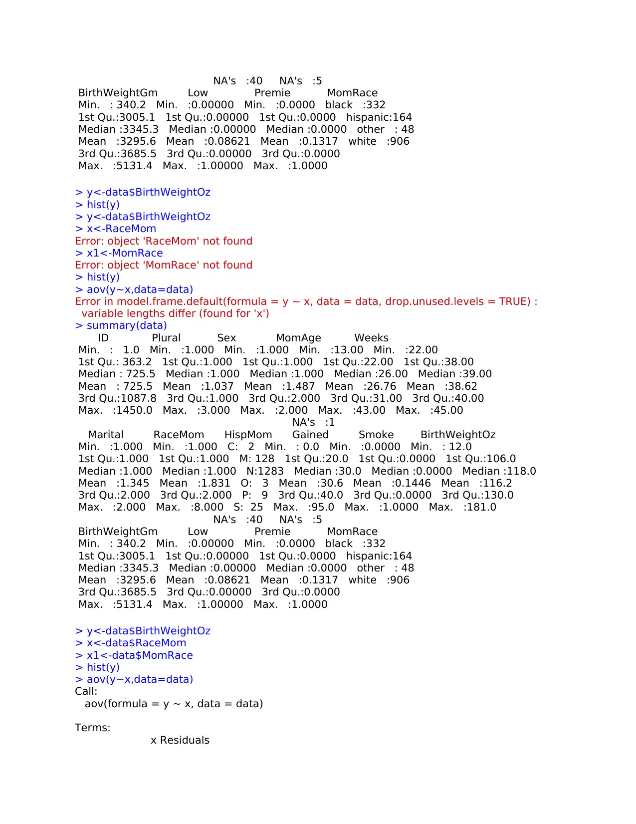
NA's :40 NA's :5
BirthWeightGm Low Premie MomRace
Min. : 340.2 Min. :0.00000 Min. :0.0000 black :332
1st Qu.:3005.1 1st Qu.:0.00000 1st Qu.:0.0000 hispanic:164
Median :3345.3 Median :0.00000 Median :0.0000 other : 48
Mean :3295.6 Mean :0.08621 Mean :0.1317 white :906
3rd Qu.:3685.5 3rd Qu.:0.00000 3rd Qu.:0.0000
Max. :5131.4 Max. :1.00000 Max. :1.0000
> y<-data$BirthWeightOz
> hist(y)
> y<-data$BirthWeightOz
> x<-RaceMom
Error: object 'RaceMom' not found
> x1<-MomRace
Error: object 'MomRace' not found
> hist(y)
> aov(y~x,data=data)
Error in model.frame.default(formula = y ~ x, data = data, drop.unused.levels = TRUE) :
variable lengths differ (found for 'x')
> summary(data)
ID Plural Sex MomAge Weeks
Min. : 1.0 Min. :1.000 Min. :1.000 Min. :13.00 Min. :22.00
1st Qu.: 363.2 1st Qu.:1.000 1st Qu.:1.000 1st Qu.:22.00 1st Qu.:38.00
Median : 725.5 Median :1.000 Median :1.000 Median :26.00 Median :39.00
Mean : 725.5 Mean :1.037 Mean :1.487 Mean :26.76 Mean :38.62
3rd Qu.:1087.8 3rd Qu.:1.000 3rd Qu.:2.000 3rd Qu.:31.00 3rd Qu.:40.00
Max. :1450.0 Max. :3.000 Max. :2.000 Max. :43.00 Max. :45.00
NA's :1
Marital RaceMom HispMom Gained Smoke BirthWeightOz
Min. :1.000 Min. :1.000 C: 2 Min. : 0.0 Min. :0.0000 Min. : 12.0
1st Qu.:1.000 1st Qu.:1.000 M: 128 1st Qu.:20.0 1st Qu.:0.0000 1st Qu.:106.0
Median :1.000 Median :1.000 N:1283 Median :30.0 Median :0.0000 Median :118.0
Mean :1.345 Mean :1.831 O: 3 Mean :30.6 Mean :0.1446 Mean :116.2
3rd Qu.:2.000 3rd Qu.:2.000 P: 9 3rd Qu.:40.0 3rd Qu.:0.0000 3rd Qu.:130.0
Max. :2.000 Max. :8.000 S: 25 Max. :95.0 Max. :1.0000 Max. :181.0
NA's :40 NA's :5
BirthWeightGm Low Premie MomRace
Min. : 340.2 Min. :0.00000 Min. :0.0000 black :332
1st Qu.:3005.1 1st Qu.:0.00000 1st Qu.:0.0000 hispanic:164
Median :3345.3 Median :0.00000 Median :0.0000 other : 48
Mean :3295.6 Mean :0.08621 Mean :0.1317 white :906
3rd Qu.:3685.5 3rd Qu.:0.00000 3rd Qu.:0.0000
Max. :5131.4 Max. :1.00000 Max. :1.0000
> y<-data$BirthWeightOz
> x<-data$RaceMom
> x1<-data$MomRace
> hist(y)
> aov(y~x,data=data)
Call:
aov(formula = y ~ x, data = data)
Terms:
x Residuals

Sum of Squares 0.8 722333.3
Deg. of Freedom 1 1448
Residual standard error: 22.33493
Estimated effects may be unbalanced
> aov(y~x1,data=data)
Call:
aov(formula = y ~ x1, data = data)
Terms:
x1 Residuals
Sum of Squares 14002.4 708331.7
Deg. of Freedom 3 1446
Residual standard error: 22.13269
Estimated effects may be unbalanced
> reg<-lm(y~x1)
> anova(reg)
Analysis of Variance Table
Response: y
Df Sum Sq Mean Sq F value Pr(>F)
x1 3 14002 4667.5 9.5282 3.118e-06 ***
Residuals 1446 708332 489.9
---
Signif. codes: 0 ‘***’ 0.001 ‘**’ 0.01 ‘*’ 0.05 ‘.’ 0.1 ‘ ’ 1
> data<-read.csv(file.choose(),header=T)
> summary(data)
Ht4 Acid Row
Min. :0.45 1.5HCl:5 a:3
1st Qu.:1.05 3.0HCl:5 b:3
Median :1.45 water :5 c:3
Mean :1.74 d:3
3rd Qu.:2.13 e:3
Max. :4.85
> mean(row,Ht4)
[1] NA
Warning message:
In mean.default(row, Ht4) :
argument is not numeric or logical: returning NA
> head(data)
Ht4 Acid Row
1 1.45 water a
2 2.79 water b
3 1.93 water c
4 2.33 water d
5 4.85 water e
6 1.00 1.5HCl a
> model<-aov( Ht4~Acid+Row,data=data)
> summary(model)
Df Sum Sq Mean Sq F value Pr(>F)
Acid 2 6.852 3.426 4.513 0.0487
Row 4 4.183 1.046 1.378 0.3235
Residuals 8 6.072 0.759

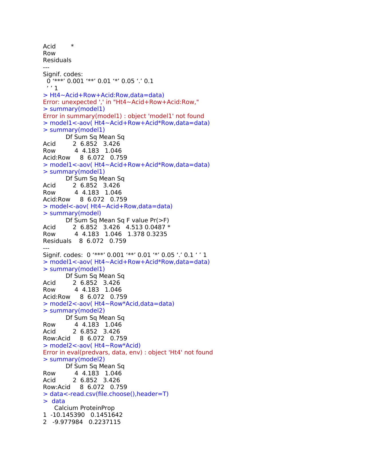
Acid *
Row
Residuals
---
Signif. codes:
0 ‘***’ 0.001 ‘**’ 0.01 ‘*’ 0.05 ‘.’ 0.1
‘ ’ 1
> Ht4~Acid+Row+Acid:Row,data=data)
Error: unexpected ',' in "Ht4~Acid+Row+Acid:Row,"
> summary(model1)
Error in summary(model1) : object 'model1' not found
> model1<-aov( Ht4~Acid+Row+Acid*Row,data=data)
> summary(model1)
Df Sum Sq Mean Sq
Acid 2 6.852 3.426
Row 4 4.183 1.046
Acid:Row 8 6.072 0.759
> model1<-aov( Ht4~Acid+Row+Acid*Row,data=data)
> summary(model1)
Df Sum Sq Mean Sq
Acid 2 6.852 3.426
Row 4 4.183 1.046
Acid:Row 8 6.072 0.759
> model<-aov( Ht4~Acid+Row,data=data)
> summary(model)
Df Sum Sq Mean Sq F value Pr(>F)
Acid 2 6.852 3.426 4.513 0.0487 *
Row 4 4.183 1.046 1.378 0.3235
Residuals 8 6.072 0.759
---
Signif. codes: 0 ‘***’ 0.001 ‘**’ 0.01 ‘*’ 0.05 ‘.’ 0.1 ‘ ’ 1
> model1<-aov( Ht4~Acid+Row+Acid*Row,data=data)
> summary(model1)
Df Sum Sq Mean Sq
Acid 2 6.852 3.426
Row 4 4.183 1.046
Acid:Row 8 6.072 0.759
> model2<-aov( Ht4~Row*Acid,data=data)
> summary(model2)
Df Sum Sq Mean Sq
Row 4 4.183 1.046
Acid 2 6.852 3.426
Row:Acid 8 6.072 0.759
> model2<-aov( Ht4~Row*Acid)
Error in eval(predvars, data, env) : object 'Ht4' not found
> summary(model2)
Df Sum Sq Mean Sq
Row 4 4.183 1.046
Acid 2 6.852 3.426
Row:Acid 8 6.072 0.759
> data<-read.csv(file.choose(),header=T)
> data
Calcium ProteinProp
1 -10.145390 0.1451642
2 -9.977984 0.2237115

3 -9.351250 0.2198288
4 -9.101001 0.3342694
5 -9.013766 0.3785262
6 -8.940437 0.4093691
7 -8.578232 0.5074450
8 -8.370183 0.5716413
9 -8.289037 0.6421870
10 -7.959793 0.8072800
11 -7.592269 0.9300252
12 -7.238448 0.9014096
13 -7.038626 0.9503276
14 -6.330776 0.9573205
15 -6.167236 0.9851045
16 -5.556894 0.9694070
17 -5.321209 0.9992852
18 -4.813609 1.0000000
19 -10.145390 0.1882841
20 -9.977984 0.2268408
21 -9.351250 0.2998251
22 -9.101001 0.3517163
23 -9.013766 0.4139161
24 -8.940437 0.4374755
25 -8.578232 0.5263771
26 -8.370183 0.6197400
27 -8.289037 0.6709965
28 -7.959793 0.8444435
29 -7.592269 0.9298122
30 -7.238448 0.9798032
31 -7.038626 0.9742129
32 -6.330776 0.9742309
33 -6.167236 0.9875247
34 -5.556894 0.9982300
35 -5.321209 1.0000000
36 -4.813609 0.9957145
37 -10.721933 0.2647664
38 -10.445753 0.3369681
39 -9.689732 0.4011040
40 -9.047837 0.3971727
41 -8.791559 0.5356422
42 -8.448916 0.6486877
43 -8.088203 0.6680274
44 -7.851397 0.8055475
45 -7.658565 0.8586845
46 -7.482276 0.8798047
47 -7.306449 1.0000000
48 -7.115545 0.9771862
49 -6.884057 0.9651696
50 -6.539854 0.9645220
51 -5.865186 0.9858963
> x<-data$Calcium
> y<-data$ProteinProp
> model<-lm( y~ poly(x, degree=3))
> model
Call:

lm(formula = y ~ poly(x, degree = 3))
Coefficients:
(Intercept) poly(x, degree = 3)1 poly(x, degree = 3)2 poly(x, degree = 3)3
0.6871 1.8962 -0.4988 -0.4673
> plot(x,y)
> plot(x,y,col='deepskyblue4',xlab='Calcium', ylab='ProteinProp',main='ProteinProp
against Calcium ')
> xsq<-x*x
> xcub<-x*x*x
> fit2<-lm(y~x+xsq)
> fit3<-lm(y~x+xsq+xcub)
> xv<-seq(min(x),max(x),0.01)
> yv<-predict(fit3,list(x=xv,xsq=xv^2,xcub=xv^3))
> lines(xv,yv,col="black")
> summary(model)
Call:
lm(formula = y ~ poly(x, degree = 3))
Residuals:
Min 1Q Median 3Q Max
-0.14031 -0.05528 -0.01859 0.05267 0.13583
Coefficients:
Estimate Std. Error t value Pr(>|t|)
(Intercept) 0.68707 0.00994 69.120 < 2e-16 ***
poly(x, degree = 3)1 1.89623 0.07099 26.712 < 2e-16 ***
poly(x, degree = 3)2 -0.49882 0.07099 -7.027 7.44e-09 ***
poly(x, degree = 3)3 -0.46729 0.07099 -6.583 3.51e-08 ***
---
Signif. codes: 0 ‘***’ 0.001 ‘**’ 0.01 ‘*’ 0.05 ‘.’ 0.1 ‘ ’ 1
Residual standard error: 0.07099 on 47 degrees of freedom
Multiple R-squared: 0.9449, Adjusted R-squared: 0.9414
F-statistic: 268.8 on 3 and 47 DF, p-value: < 2.2e-16
> data<-read.csv(file.choose(),header=T)
> x<-data$Elevation
> y<-data$Time
> z<-data$Length
> plot(x,y,col='deepskyblue4',xlab='Elevation (in feet)',ylab='Time (in hours)',main='Time
against Elevation')
> cor(x,y)
[1] -0.0162768
> model<-lm(y~x+z)
> summary(model)
Call:
lm(formula = y ~ x + z)
Residuals:
Min 1Q Median 3Q Max
-2.5924 -0.8050 -0.1959 0.6380 3.8432

Coefficients:
Estimate Std. Error t value Pr(>|t|)
(Intercept) 8.0753787 2.5327132 3.188 0.00267 **
x -0.0014483 0.0005805 -2.495 0.01653 *
z 0.7123344 0.0593330 12.006 2.54e-15 ***
---
Signif. codes: 0 ‘***’ 0.001 ‘**’ 0.01 ‘*’ 0.05 ‘.’ 0.1 ‘ ’ 1
Residual standard error: 1.37 on 43 degrees of freedom
Multiple R-squared: 0.7703, Adjusted R-squared: 0.7596
F-statistic: 72.09 on 2 and 43 DF, p-value: 1.844e-14
> summary(lm(y~x))
Call:
lm(formula = y ~ x)
Residuals:
Min 1Q Median 3Q Max
-5.6912 -1.6985 -0.5639 1.2963 7.3015
Coefficients:
Estimate Std. Error t value Pr(>|t|)
(Intercept) 11.2113764 5.1953800 2.158 0.0364 *
x -0.0001269 0.0011756 -0.108 0.9145
---
Signif. codes: 0 ‘***’ 0.001 ‘**’ 0.01 ‘*’ 0.05 ‘.’ 0.1 ‘ ’ 1
Residual standard error: 2.826 on 44 degrees of freedom
Multiple R-squared: 0.0002649, Adjusted R-squared: -0.02246
F-statistic: 0.01166 on 1 and 44 DF, p-value: 0.9145
> summary(lm(y~z))
Call:
lm(formula = y ~ z)
Residuals:
Min 1Q Median 3Q Max
-2.4491 -0.6687 -0.0122 0.5590 4.0034
Coefficients:
Estimate Std. Error t value Pr(>|t|)
(Intercept) 2.04817 0.80371 2.548 0.0144 *
z 0.68427 0.06162 11.105 2.39e-14 ***
---
Signif. codes: 0 ‘***’ 0.001 ‘**’ 0.01 ‘*’ 0.05 ‘.’ 0.1 ‘ ’ 1
Residual standard error: 1.449 on 44 degrees of freedom
Multiple R-squared: 0.737, Adjusted R-squared: 0.7311
F-statistic: 123.3 on 1 and 44 DF, p-value: 2.39e-14
> r1<-lm(y~z)
> r2<-lm(x~z)

> plot(r1 $residuals,r2 $residuals,main="r2 $residuals versus r1residuals")
> lm(r1 $residuals,r2 $residuals)
Error in formula.default(object, env = baseenv()) : invalid formula
> r3
Error: object 'r3' not found
> summary(r3)
Error in summary(r3) : object 'r3' not found
> data<-read.csv(file.choose(),header=T)
> summary(data)
ID Plural Sex MomAge Weeks
Min. : 1.0 Min. :1.000 Min. :1.000 Min. :13.00 Min. :22.00
1st Qu.: 363.2 1st Qu.:1.000 1st Qu.:1.000 1st Qu.:22.00 1st Qu.:38.00
Median : 725.5 Median :1.000 Median :1.000 Median :26.00 Median :39.00
Mean : 725.5 Mean :1.037 Mean :1.487 Mean :26.76 Mean :38.62
3rd Qu.:1087.8 3rd Qu.:1.000 3rd Qu.:2.000 3rd Qu.:31.00 3rd Qu.:40.00
Max. :1450.0 Max. :3.000 Max. :2.000 Max. :43.00 Max. :45.00
NA's :1
Marital RaceMom HispMom Gained Smoke BirthWeightOz
Min. :1.000 Min. :1.000 C: 2 Min. : 0.0 Min. :0.0000 Min. : 12.0
1st Qu.:1.000 1st Qu.:1.000 M: 128 1st Qu.:20.0 1st Qu.:0.0000 1st Qu.:106.0
Median :1.000 Median :1.000 N:1283 Median :30.0 Median :0.0000 Median :118.0
Mean :1.345 Mean :1.831 O: 3 Mean :30.6 Mean :0.1446 Mean :116.2
3rd Qu.:2.000 3rd Qu.:2.000 P: 9 3rd Qu.:40.0 3rd Qu.:0.0000 3rd Qu.:130.0
Max. :2.000 Max. :8.000 S: 25 Max. :95.0 Max. :1.0000 Max. :181.0
NA's :40 NA's :5
BirthWeightGm Low Premie MomRace
Min. : 340.2 Min. :0.00000 Min. :0.0000 black :332
1st Qu.:3005.1 1st Qu.:0.00000 1st Qu.:0.0000 hispanic:164
Median :3345.3 Median :0.00000 Median :0.0000 other : 48
Mean :3295.6 Mean :0.08621 Mean :0.1317 white :906
3rd Qu.:3685.5 3rd Qu.:0.00000 3rd Qu.:0.0000
Max. :5131.4 Max. :1.00000 Max. :1.0000
> y<-data$BirthWeightOz
> x<-data$RaceMom
> x1<-data$MomRace
> hist(y)
> aov(y~x,data=data)
Call:
aov(formula = y ~ x, data = data)
Terms:
x Residuals
Sum of Squares 0.8 722333.3
Deg. of Freedom 1 1448
Residual standard error: 22.33493
Estimated effects may be unbalanced
> aov(y~x1,data=data)
Call:
aov(formula = y ~ x1, data = data)
Terms:
x1 Residuals
Sum of Squares 14002.4 708331.7

Deg. of Freedom 3 1446
Residual standard error: 22.13269
Estimated effects may be unbalanced
> reg<-lm(y~x1)
> anova(reg)
Analysis of Variance Table
Response: y
Df Sum Sq Mean Sq F value Pr(>F)
x1 3 14002 4667.5 9.5282 3.118e-06 ***
Residuals 1446 708332 489.9
---
Signif. codes: 0 ‘***’ 0.001 ‘**’ 0.01 ‘*’ 0.05 ‘.’ 0.1 ‘ ’ 1
> data<-read.csv(file.choose(),header=T)
> model<-aov( Ht4~Acid+Row,data=data)
> summary(model)
Df Sum Sq Mean Sq F value Pr(>F)
Acid 2 6.852 3.426 4.513 0.0487 *
Row 4 4.183 1.046 1.378 0.3235
Residuals 8 6.072 0.759
---
Signif. codes: 0 ‘***’ 0.001 ‘**’ 0.01 ‘*’ 0.05 ‘.’ 0.1 ‘ ’ 1
> model1<-aov( Ht4~Acid+Row+Acid*Row,data=data)
> summary(model1)
Df Sum Sq Mean Sq
Acid 2 6.852 3.426
Row 4 4.183 1.046
Acid:Row 8 6.072 0.759
> model2<-aov( Ht4~Row*Acid,data=data)
> summary(model2)
Df Sum Sq Mean Sq
Row 4 4.183 1.046
Acid 2 6.852 3.426
Row:Acid 8 6.072 0.759