Statistical Analysis and Regression for Business Data - Assignment

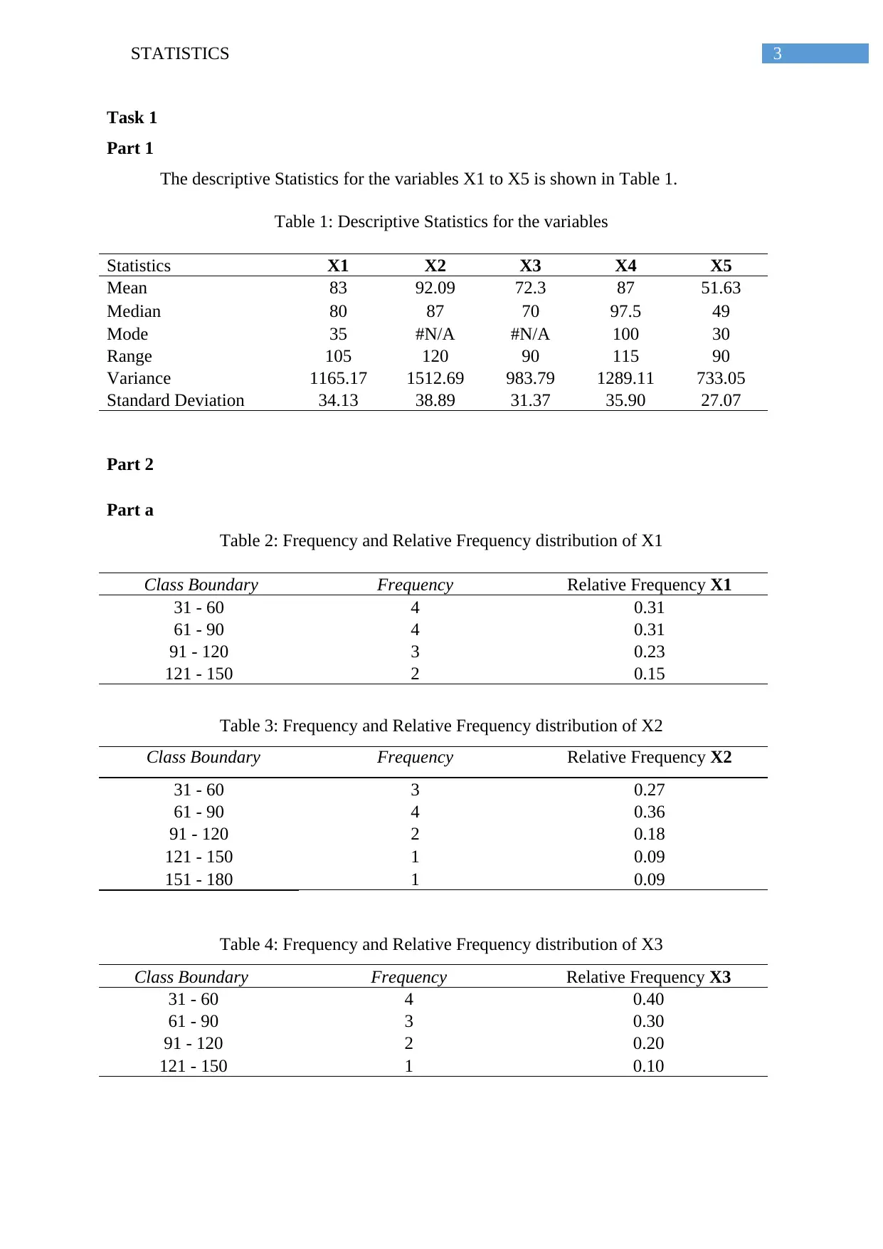
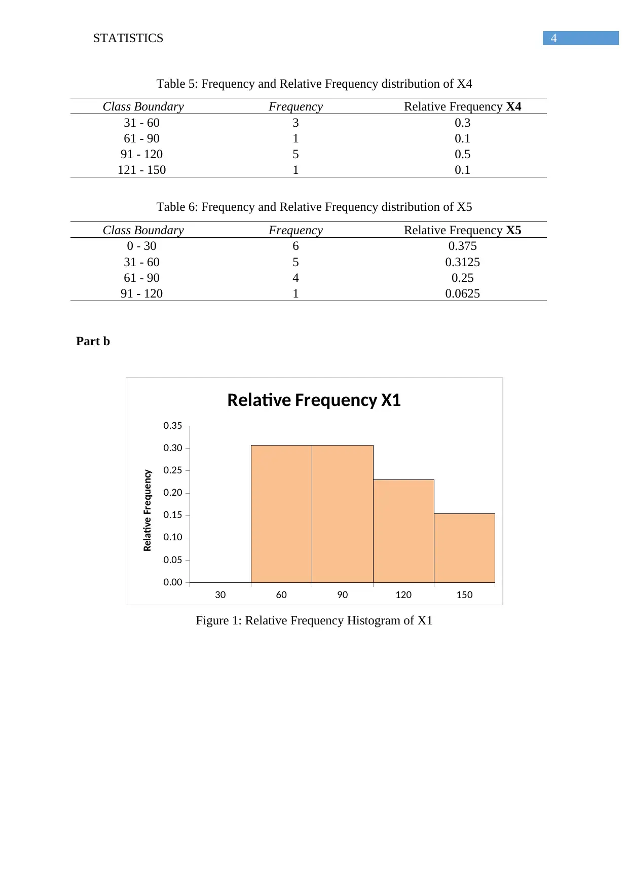
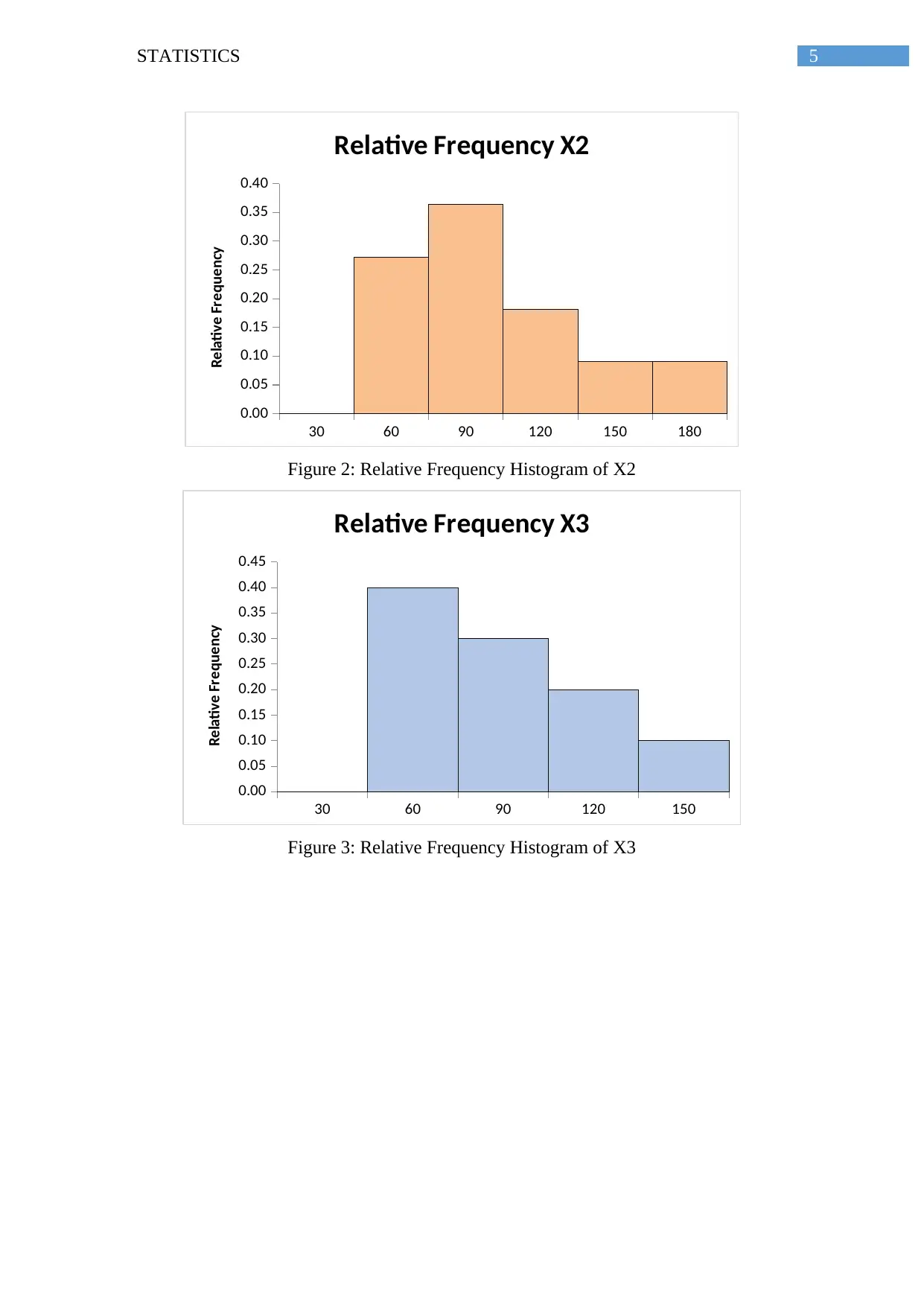
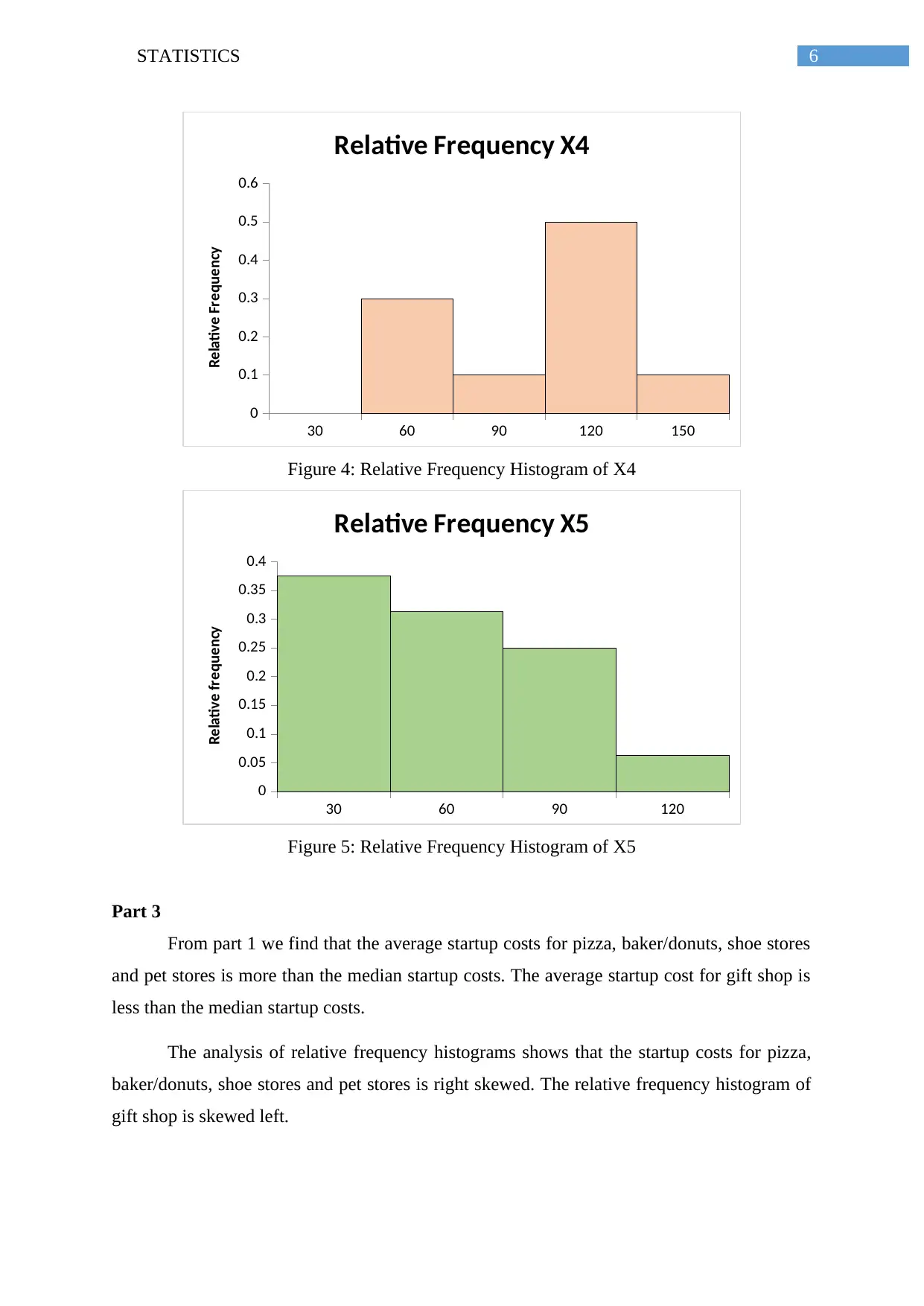
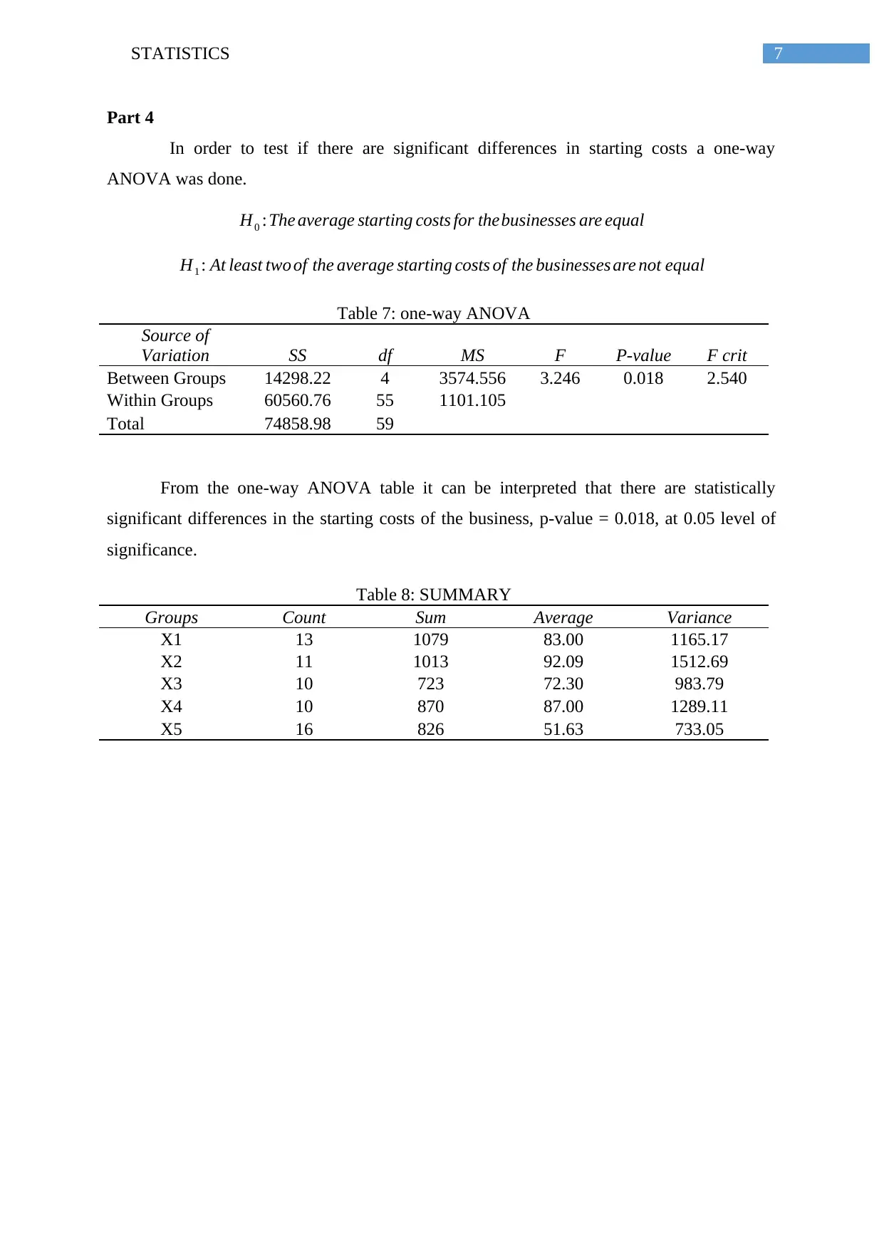
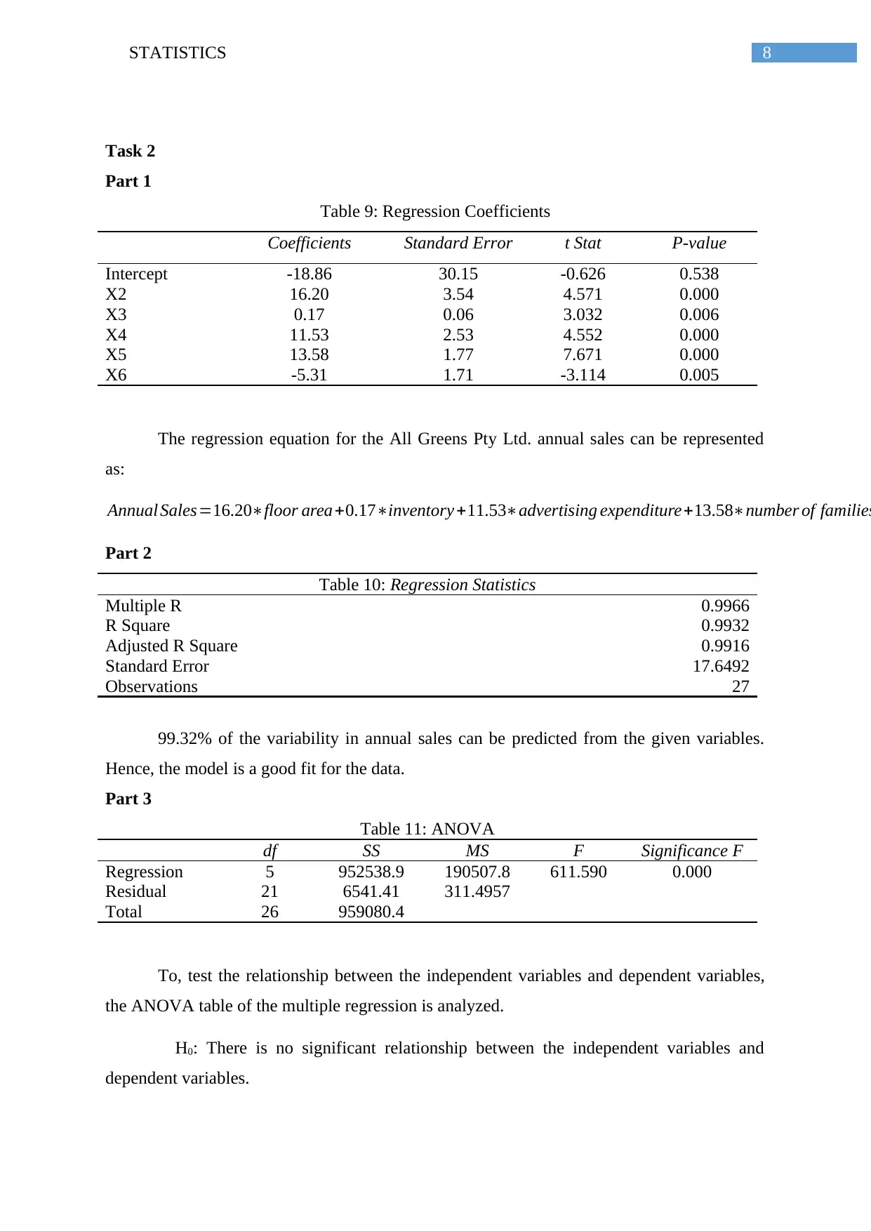
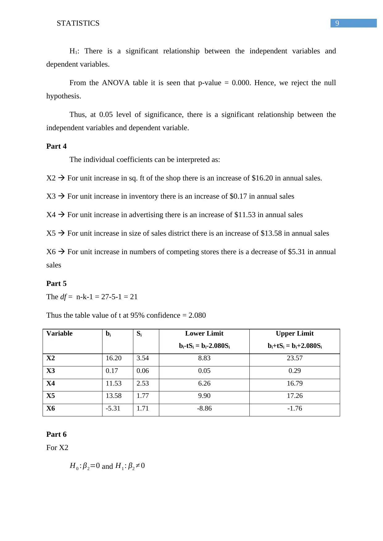
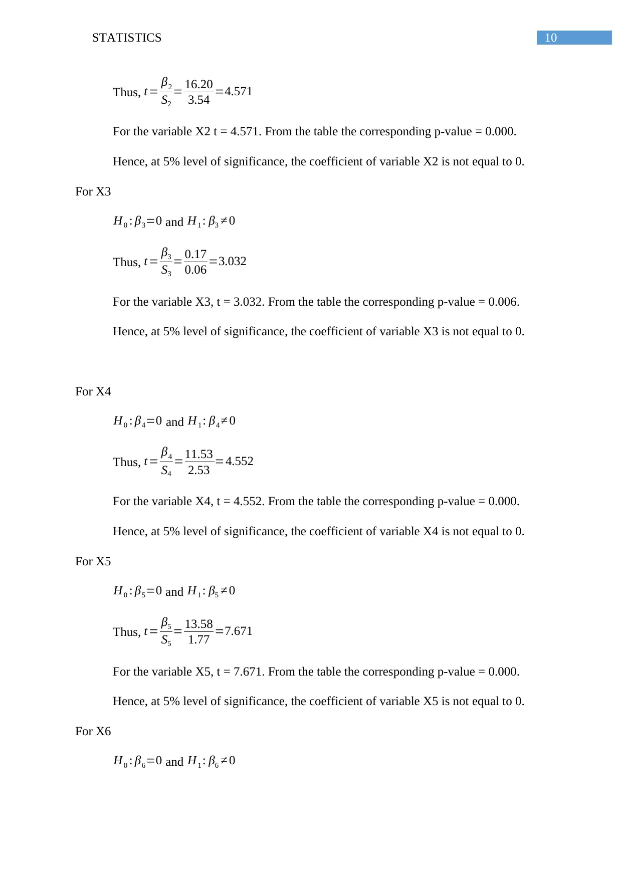
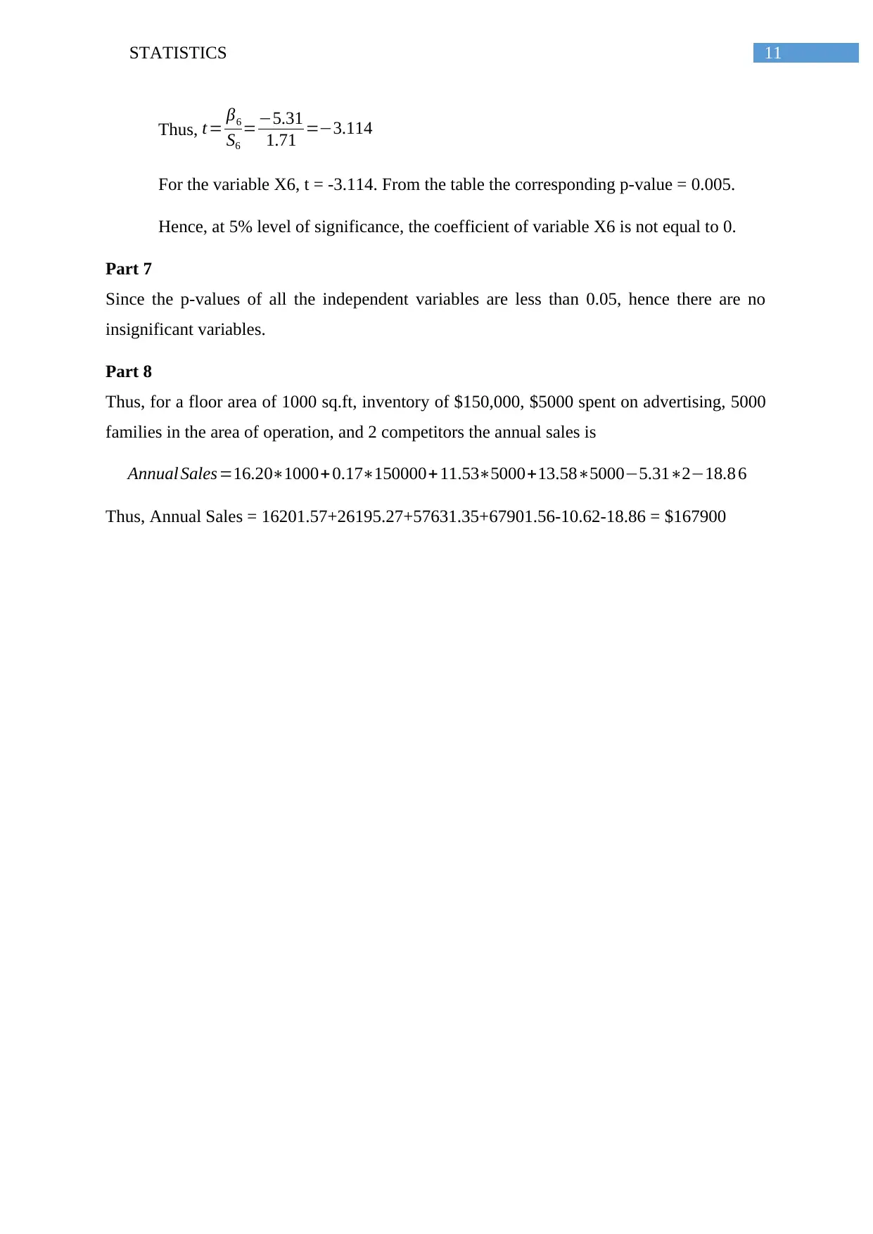
This statistics assignment presents a comprehensive analysis of business data, encompassing descriptive statistics, frequency distributions, and regression analysis. The assignment begins with calculating descriptive statistics (mean, median, mode, range, variance, and standard deviation) for multiple variables. It then delves into frequency and relative frequency distributions, visualized through histograms, to understand data patterns. The analysis extends to hypothesis testing using one-way ANOVA to determine significant differences in startup costs. Furthermore, the assignment explores multiple regression analysis, interpreting coefficients, assessing model fit, and conducting t-tests for individual coefficients to evaluate the impact of various factors on annual sales. The solution provides a step-by-step breakdown of calculations, interpretations, and conclusions, offering a valuable resource for students studying statistical methods and their application in business contexts.

Running head: STATISTICS
Statistics
Name of the Student
Name of the University
Author Note

2STATISTICS
Table of Contents
Task 1.........................................................................................................................................3
Part 1......................................................................................................................................3
Part 2......................................................................................................................................3
Part a...................................................................................................................................3
Part b..................................................................................................................................4
Part 3......................................................................................................................................6
Part 4......................................................................................................................................7
Task 2.........................................................................................................................................8
Part 1......................................................................................................................................8
Part 2......................................................................................................................................8
Part 3......................................................................................................................................8
Part 4......................................................................................................................................9
Part 5......................................................................................................................................9
Part 6......................................................................................................................................9
Part 7....................................................................................................................................11
Part 8....................................................................................................................................11

3STATISTICS
Task 1
Part 1
The descriptive Statistics for the variables X1 to X5 is shown in Table 1.
Table 1: Descriptive Statistics for the variables
Statistics X1 X2 X3 X4 X5
Mean 83 92.09 72.3 87 51.63
Median 80 87 70 97.5 49
Mode 35 #N/A #N/A 100 30
Range 105 120 90 115 90
Variance 1165.17 1512.69 983.79 1289.11 733.05
Standard Deviation 34.13 38.89 31.37 35.90 27.07
Part 2
Part a
Table 2: Frequency and Relative Frequency distribution of X1
Class Boundary Frequency Relative Frequency X1
31 - 60 4 0.31
61 - 90 4 0.31
91 - 120 3 0.23
121 - 150 2 0.15
Table 3: Frequency and Relative Frequency distribution of X2
Class Boundary Frequency Relative Frequency X2
31 - 60 3 0.27
61 - 90 4 0.36
91 - 120 2 0.18
121 - 150 1 0.09
151 - 180 1 0.09
Table 4: Frequency and Relative Frequency distribution of X3
Class Boundary Frequency Relative Frequency X3
31 - 60 4 0.40
61 - 90 3 0.30
91 - 120 2 0.20
121 - 150 1 0.10

4STATISTICS
Table 5: Frequency and Relative Frequency distribution of X4
Class Boundary Frequency Relative Frequency X4
31 - 60 3 0.3
61 - 90 1 0.1
91 - 120 5 0.5
121 - 150 1 0.1
Table 6: Frequency and Relative Frequency distribution of X5
Class Boundary Frequency Relative Frequency X5
0 - 30 6 0.375
31 - 60 5 0.3125
61 - 90 4 0.25
91 - 120 1 0.0625
Part b
30 60 90 120 150
0.00
0.05
0.10
0.15
0.20
0.25
0.30
0.35
Relative Frequency X1
Relative Frequency
Figure 1: Relative Frequency Histogram of X1

5STATISTICS
30 60 90 120 150 180
0.00
0.05
0.10
0.15
0.20
0.25
0.30
0.35
0.40
Relative Frequency X2
Relative Frequency
Figure 2: Relative Frequency Histogram of X2
30 60 90 120 150
0.00
0.05
0.10
0.15
0.20
0.25
0.30
0.35
0.40
0.45
Relative Frequency X3
Relative Frequency
Figure 3: Relative Frequency Histogram of X3

6STATISTICS
30 60 90 120 150
0
0.1
0.2
0.3
0.4
0.5
0.6
Relative Frequency X4
Relative Frequency
Figure 4: Relative Frequency Histogram of X4
30 60 90 120
0
0.05
0.1
0.15
0.2
0.25
0.3
0.35
0.4
Relative Frequency X5
Relative frequency
Figure 5: Relative Frequency Histogram of X5
Part 3
From part 1 we find that the average startup costs for pizza, baker/donuts, shoe stores
and pet stores is more than the median startup costs. The average startup cost for gift shop is
less than the median startup costs.
The analysis of relative frequency histograms shows that the startup costs for pizza,
baker/donuts, shoe stores and pet stores is right skewed. The relative frequency histogram of
gift shop is skewed left.

7STATISTICS
Part 4
In order to test if there are significant differences in starting costs a one-way
ANOVA was done.
H0 :The average starting costs for thebusinesses are equal
H1 : At least two of the average starting costs of the businesses are not equal
Table 7: one-way ANOVA
Source of
Variation SS df MS F P-value F crit
Between Groups 14298.22 4 3574.556 3.246 0.018 2.540
Within Groups 60560.76 55 1101.105
Total 74858.98 59
From the one-way ANOVA table it can be interpreted that there are statistically
significant differences in the starting costs of the business, p-value = 0.018, at 0.05 level of
significance.
Table 8: SUMMARY
Groups Count Sum Average Variance
X1 13 1079 83.00 1165.17
X2 11 1013 92.09 1512.69
X3 10 723 72.30 983.79
X4 10 870 87.00 1289.11
X5 16 826 51.63 733.05

8STATISTICS
Task 2
Part 1
Table 9: Regression Coefficients
Coefficients Standard Error t Stat P-value
Intercept -18.86 30.15 -0.626 0.538
X2 16.20 3.54 4.571 0.000
X3 0.17 0.06 3.032 0.006
X4 11.53 2.53 4.552 0.000
X5 13.58 1.77 7.671 0.000
X6 -5.31 1.71 -3.114 0.005
The regression equation for the All Greens Pty Ltd. annual sales can be represented
as:
Annual Sales=16.20∗floor area+0.17∗inventory +11.53∗advertising expenditure+13.58∗number of families
Part 2
Table 10: Regression Statistics
Multiple R 0.9966
R Square 0.9932
Adjusted R Square 0.9916
Standard Error 17.6492
Observations 27
99.32% of the variability in annual sales can be predicted from the given variables.
Hence, the model is a good fit for the data.
Part 3
Table 11: ANOVA
df SS MS F Significance F
Regression 5 952538.9 190507.8 611.590 0.000
Residual 21 6541.41 311.4957
Total 26 959080.4
To, test the relationship between the independent variables and dependent variables,
the ANOVA table of the multiple regression is analyzed.
H0: There is no significant relationship between the independent variables and
dependent variables.

9STATISTICS
H1: There is a significant relationship between the independent variables and
dependent variables.
From the ANOVA table it is seen that p-value = 0.000. Hence, we reject the null
hypothesis.
Thus, at 0.05 level of significance, there is a significant relationship between the
independent variables and dependent variable.
Part 4
The individual coefficients can be interpreted as:
X2  For unit increase in sq. ft of the shop there is an increase of $16.20 in annual sales.
X3  For unit increase in inventory there is an increase of $0.17 in annual sales
X4  For unit increase in advertising there is an increase of $11.53 in annual sales
X5  For unit increase in size of sales district there is an increase of $13.58 in annual sales
X6  For unit increase in numbers of competing stores there is a decrease of $5.31 in annual
sales
Part 5
The df = n-k-1 = 27-5-1 = 21
Thus the table value of t at 95% confidence = 2.080
Variable bi Si Lower Limit
bi-tSi = bi-2.080Si
Upper Limit
bi+tSi = bi+2.080Si
X2 16.20 3.54 8.83 23.57
X3 0.17 0.06 0.05 0.29
X4 11.53 2.53 6.26 16.79
X5 13.58 1.77 9.90 17.26
X6 -5.31 1.71 -8.86 -1.76
Part 6
For X2
H0 : β2=0 and H1 : β2 ≠ 0

10STATISTICS
Thus, t= β2
S2
= 16.20
3.54 =4.571
For the variable X2 t = 4.571. From the table the corresponding p-value = 0.000.
Hence, at 5% level of significance, the coefficient of variable X2 is not equal to 0.
For X3
H0 : β3=0 and H1 : β3 ≠ 0
Thus, t= β3
S3
= 0.17
0.06 =3.032
For the variable X3, t = 3.032. From the table the corresponding p-value = 0.006.
Hence, at 5% level of significance, the coefficient of variable X3 is not equal to 0.
For X4
H0 : β4=0 and H1 : β4 ≠ 0
Thus, t= β4
S4
=11.53
2.53 =4.552
For the variable X4, t = 4.552. From the table the corresponding p-value = 0.000.
Hence, at 5% level of significance, the coefficient of variable X4 is not equal to 0.
For X5
H0 : β5=0 and H1 : β5 ≠ 0
Thus, t= β5
S5
= 13.58
1.77 =7.671
For the variable X5, t = 7.671. From the table the corresponding p-value = 0.000.
Hence, at 5% level of significance, the coefficient of variable X5 is not equal to 0.
For X6
H0 : β6=0 and H1 : β6 ≠ 0

11STATISTICS
Thus, t= β6
S6
=−5.31
1.71 =−3.114
For the variable X6, t = -3.114. From the table the corresponding p-value = 0.005.
Hence, at 5% level of significance, the coefficient of variable X6 is not equal to 0.
Part 7
Since the p-values of all the independent variables are less than 0.05, hence there are no
insignificant variables.
Part 8
Thus, for a floor area of 1000 sq.ft, inventory of $150,000, $5000 spent on advertising, 5000
families in the area of operation, and 2 competitors the annual sales is
Annual Sales=16.20∗1000+ 0.17∗150000+ 11.53∗5000+13.58∗5000−5.31∗2−18.8 6
Thus, Annual Sales = 16201.57+26195.27+57631.35+67901.56-10.62-18.86 = $167900