Statistics Assignment: Brain Size, Infection Risk, Medical Expenses

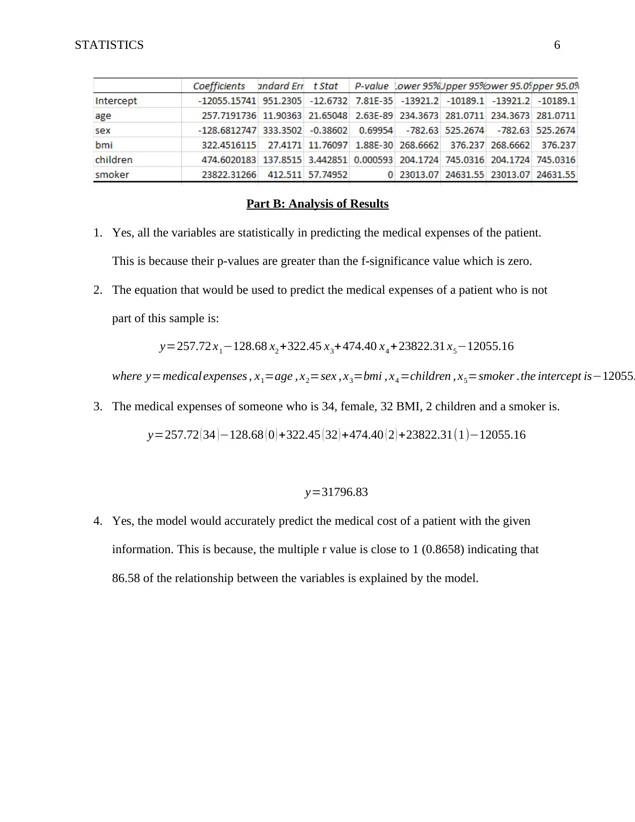
This statistics assignment delves into exploratory data analysis and regression models across three distinct scenarios. The first part involves analyzing brain size data, computing a five-number summary, identifying outliers, and assessing the relationship between head size and brain weight using Excel. The second part focuses on infection risk in hospitals, utilizing multiple linear regression to model the influence of various factors on patient infection. Finally, the assignment explores medical expenses, employing regression to predict costs based on patient characteristics. The student analyzes statistical significance, correlation, and the impact of outliers, providing comprehensive insights into each dataset and model.

Running head: STATISTICS 1
Statistics
Student Name
Professor’s Name
University Name
Date

STATISTICS 2
Part 1: Brain Size
Part A: Excel Task
a. We need to use excel to compute the five-number summary using the head size column.
Answer
The five-number summary include the minimum, 1st quartile, median, 3rd quartile,
and maximum (Hinton, 2014). The summary as obtained in excel for the head size
column is as shown below:
b. The interquartile range and lower/ upper limits for the outliers obtained in excel are as
shown in the figure below.
c. The maximum value is an outlier since it lies beyond the upper limit of the outlier (Evans
& Basu, 2013).
d. The scatter plot created to show the relationship between the head size and the brain
weight inclusive of the regression equation and the r-squared value is as shown below:

STATISTICS 3
e. The Residual vs. fitted plot created using the excel regression tool is as shown below:
Part B: Analysis of Results
1. The type of relationship that exist between head size and brain weight is an averagely
strong positive relationship (Freund, 2014). This is because the multiple r value is
positive and approaching 1. Moreover, the slope of the regression equation is positive.
2. The outliers of the dataset are reasonable in the sense that they are very few hence and
very close to the upper limit and hence has no huge impact on the result obtained.
Omitting the outlier is not necessarily important since it has very little impact on the
obtained result.

STATISTICS 4
3. Yes, the correlation between the two variables is significant. This is because the multiple
r value is to high (0.7995). meaning that 79.95% of the relationship between the variables
is explained by the model. The Residuals vs Fitted plot does not show a reasonable
amount of variance.
4. No, the other variables would not be significant in predicting brain weight along with
head size. This is because the they are just discrete variables used to only indicate the
either gender of an individual or the age group in which an individual exists (Croucher,
2016).
Part Two: Infection Risk in Hospitals
Part A: Excel Task
a. The mean, median, mode and standard deviation of age column is found in excel as
below:
b. The column which might influence the chance that a patient is infected while they are in
hospital are stay, age, culture, med school, region, x-ray, beds, census, nurses, and
facilities. Only the id of the patient cannot influence the chance of the patient being
infected while in hospital.
c. The multiple linear regression that creates a model that predicts the infection risk of a
patient is as shown below:

STATISTICS 5
Part B: Analysis of Results
1. The typical age of a participant of this study is the average age which is 53.2 years. The
range of patient ages that are within three standard deviations of the mean is given by:
pr (μ−3 σ ≤ x ≤ μ+3 σ )
¿ 53.23−3 ( 4.46 ) ≤ x ≤52.23+3 (4.46)
¿ 39.85 ≤ x ≤65.61
2. Yes, the regression model is a good predictor of the infection risk. This is because the
multiple r value is close to 1 (0.7548) meaning that 75.48% of the relationship between
the variables is explained by the model. All the variables selected are statistically
significant since their p-value is greater than the value of the f-significance.
Part Three: Using Medical Expenses to Project Insurance Rates
Part A: Excel Task
The mean, standard deviation, and the z score for the individual values are shown on the excel
file. Yes, there exists outliers as shown in the excel file. When the Count If function is used in
excel, there is an indication that there is a total of 138 outliers.
The regression model that predicts medical expenses by the other variables listed is as shown
below:

STATISTICS 6
Part B: Analysis of Results
1. Yes, all the variables are statistically in predicting the medical expenses of the patient.
This is because their p-values are greater than the f-significance value which is zero.
2. The equation that would be used to predict the medical expenses of a patient who is not
part of this sample is:
y=257.72 x1−128.68 x2 +322.45 x3+474.40 x4 +23822.31 x5−12055.16
where y=medical expenses , x1=age , x2=sex , x3=bmi , x4 =children , x5=smoker .the intercept is−12055.
3. The medical expenses of someone who is 34, female, 32 BMI, 2 children and a smoker is.
y=257.72 ( 34 )−128.68 ( 0 ) +322.45 ( 32 ) +474.40 ( 2 ) +23822.31(1)−12055.16
y=31796.83
4. Yes, the model would accurately predict the medical cost of a patient with the given
information. This is because, the multiple r value is close to 1 (0.8658) indicating that
86.58 of the relationship between the variables is explained by the model.

STATISTICS 7
References
Croucher, J. S. (2016). Introductory mathematics & statistics (6th ed.). Australia: North Ryde,
N.S.W. McGraw-Hill Education.
Evans, J. R., & Basu, A. (2013). Statistics, data analysis, and decision modeling (5th ed.).
Boston: Pearson.
Freund, J. E. (2014). Modern elementary statistics (12th ed.). Boston: Pearson.
Hinton, P. R. (2014). Statistics explained (3rd ed.). London: Routledge, Taylor & Francis Group.