Statistical Analysis of Data and Decision Making: Report
VerifiedAdded on 2020/07/23
|13
|2175
|47
Report
AI Summary
This report provides a comprehensive statistical analysis of various case studies, demonstrating the application of statistical tools and techniques to aid in decision-making. The report utilizes SPSS to analyze data through t-tests, regression, and correlation, addressing different hypotheses. It explores topics such as the impact of intervention programs on adolescent behavior, analysis of mean values, and the relationship between variables like weight, height, and age. The report also covers the concept of statistical significance, p-values, and cross-tabulation to assess associations between variables. Furthermore, the report provides interpretations of the statistical outputs and draws conclusions on the significance of the findings, highlighting the usefulness of statistical tools in research and analysis.
Statistics
Paraphrase This Document
Need a fresh take? Get an instant paraphrase of this document with our AI Paraphraser
TABLE OF CONTENTS
INTRODUCTION..................................................................................................................................................................1
QUESTION 1.........................................................................................................................................................................1
QUESTION 2.........................................................................................................................................................................2
QUESTION 3.........................................................................................................................................................................2
QUESTION 4.........................................................................................................................................................................2
QUESTION 5.........................................................................................................................................................................3
5.1.......................................................................................................................................................................................5
5.2.......................................................................................................................................................................................5
5.3.......................................................................................................................................................................................5
5.4.......................................................................................................................................................................................5
QUESTION 6.........................................................................................................................................................................5
QUESTION 7.........................................................................................................................................................................6
1..........................................................................................................................................................................................6
2..........................................................................................................................................................................................6
QUESTION 8.........................................................................................................................................................................6
QUESTION 9.........................................................................................................................................................................6
QUESTION 10.......................................................................................................................................................................7
QUESTION 11.......................................................................................................................................................................8
11.1.....................................................................................................................................................................................8
11.2 and 11.3....................................................................................................................................................................10
11.4...................................................................................................................................................................................12
CONCLUSION....................................................................................................................................................................13
INTRODUCTION
In the present scenario, use of statistical tools and software has increased significantly in the field of research.
SPSS tools such as chi-square, t-test, regression and correlation are highly significant which in turn provides high level
of assistance in testing hypothesis. The present report is based on different case situations which will shed light on the
manner in which different statistical tools aid in decision making.
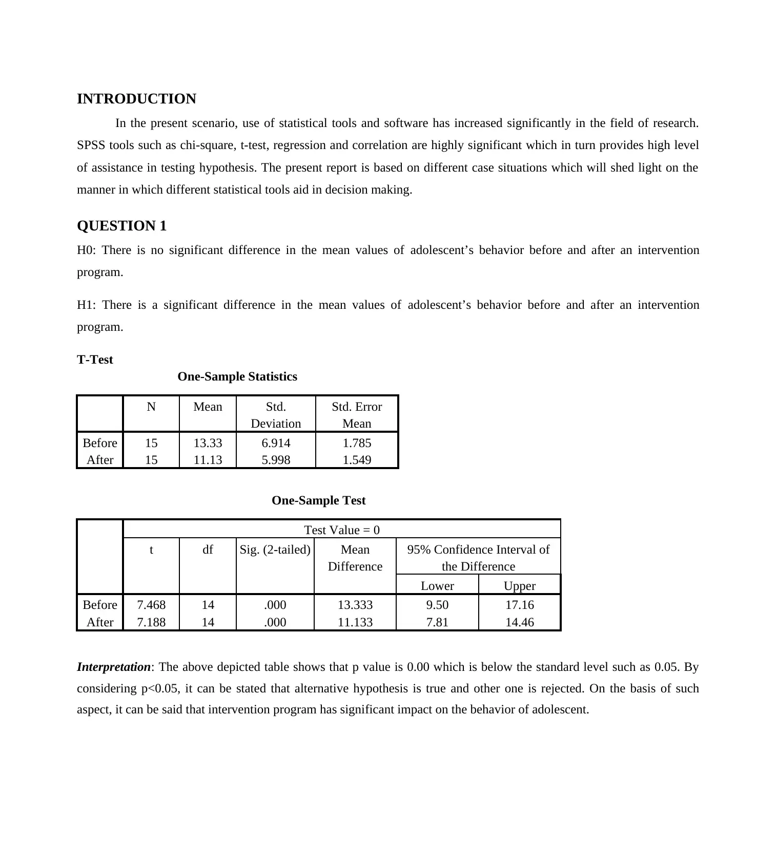
QUESTION 1
H0: There is no significant difference in the mean values of adolescent’s behavior before and after an intervention
program.
H1: There is a significant difference in the mean values of adolescent’s behavior before and after an intervention
program.
T-Test
One-Sample Statistics
N Mean Std.
Deviation
Std. Error
Mean
Before 15 13.33 6.914 1.785
After 15 11.13 5.998 1.549
One-Sample Test
Test Value = 0
t df Sig. (2-tailed) Mean
Difference
95% Confidence Interval of
the Difference
Lower Upper
Before 7.468 14 .000 13.333 9.50 17.16
After 7.188 14 .000 11.133 7.81 14.46
Interpretation: The above depicted table shows that p value is 0.00 which is below the standard level such as 0.05. By
considering p<0.05, it can be stated that alternative hypothesis is true and other one is rejected. On the basis of such
aspect, it can be said that intervention program has significant impact on the behavior of adolescent.
In the present scenario, use of statistical tools and software has increased significantly in the field of research.
SPSS tools such as chi-square, t-test, regression and correlation are highly significant which in turn provides high level
of assistance in testing hypothesis. The present report is based on different case situations which will shed light on the
manner in which different statistical tools aid in decision making.
QUESTION 1
H0: There is no significant difference in the mean values of adolescent’s behavior before and after an intervention
program.
H1: There is a significant difference in the mean values of adolescent’s behavior before and after an intervention
program.
T-Test
One-Sample Statistics
N Mean Std.
Deviation
Std. Error
Mean
Before 15 13.33 6.914 1.785
After 15 11.13 5.998 1.549
One-Sample Test
Test Value = 0
t df Sig. (2-tailed) Mean
Difference
95% Confidence Interval of
the Difference
Lower Upper
Before 7.468 14 .000 13.333 9.50 17.16
After 7.188 14 .000 11.133 7.81 14.46
Interpretation: The above depicted table shows that p value is 0.00 which is below the standard level such as 0.05. By
considering p<0.05, it can be stated that alternative hypothesis is true and other one is rejected. On the basis of such
aspect, it can be said that intervention program has significant impact on the behavior of adolescent.
⊘ This is a preview!⊘
Do you want full access?
Subscribe today to unlock all pages.
Trusted by 1+ million students worldwide
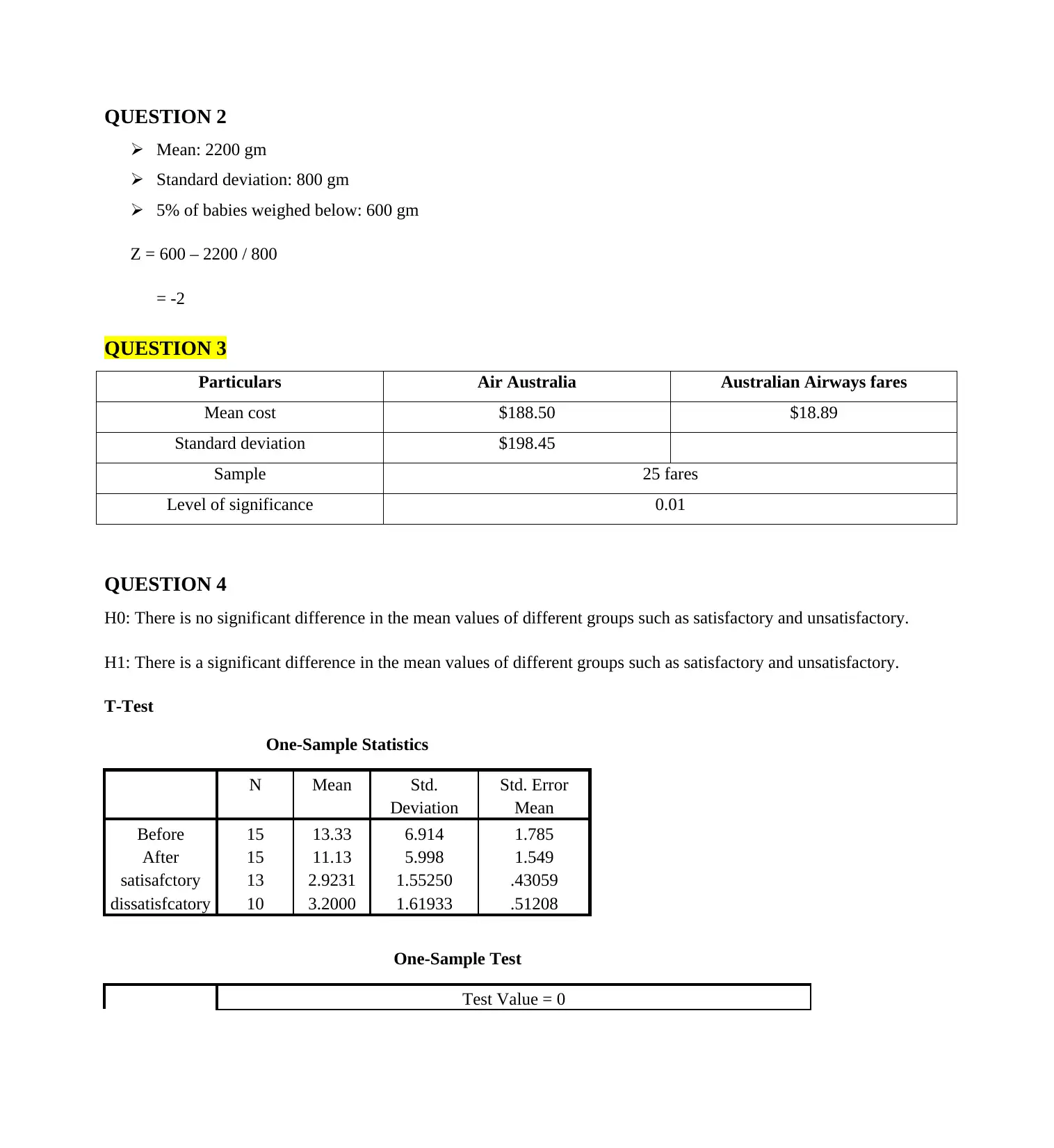
QUESTION 2
Mean: 2200 gm
Standard deviation: 800 gm
5% of babies weighed below: 600 gm
Z = 600 – 2200 / 800
= -2
QUESTION 3
Particulars Air Australia Australian Airways fares
Mean cost $188.50 $18.89
Standard deviation $198.45
Sample 25 fares
Level of significance 0.01
QUESTION 4
H0: There is no significant difference in the mean values of different groups such as satisfactory and unsatisfactory.
H1: There is a significant difference in the mean values of different groups such as satisfactory and unsatisfactory.
T-Test
One-Sample Statistics
N Mean Std.
Deviation
Std. Error
Mean
Before 15 13.33 6.914 1.785
After 15 11.13 5.998 1.549
satisafctory 13 2.9231 1.55250 .43059
dissatisfcatory 10 3.2000 1.61933 .51208
One-Sample Test
Test Value = 0
Paraphrase This Document
Need a fresh take? Get an instant paraphrase of this document with our AI Paraphraser
t df Sig. (2-tailed) Mean
Difference
95% Confidence Interval of
the Difference
Lower Upper
Before 7.468 14 .000 13.333 9.50 17.16
After 7.188 14 .000 11.133 7.81 14.46
satisafctory 6.789 12 .000 2.92308 1.9849 3.8612
dissatisfcatory 6.249 9 .000 3.20000 2.0416 4.3584
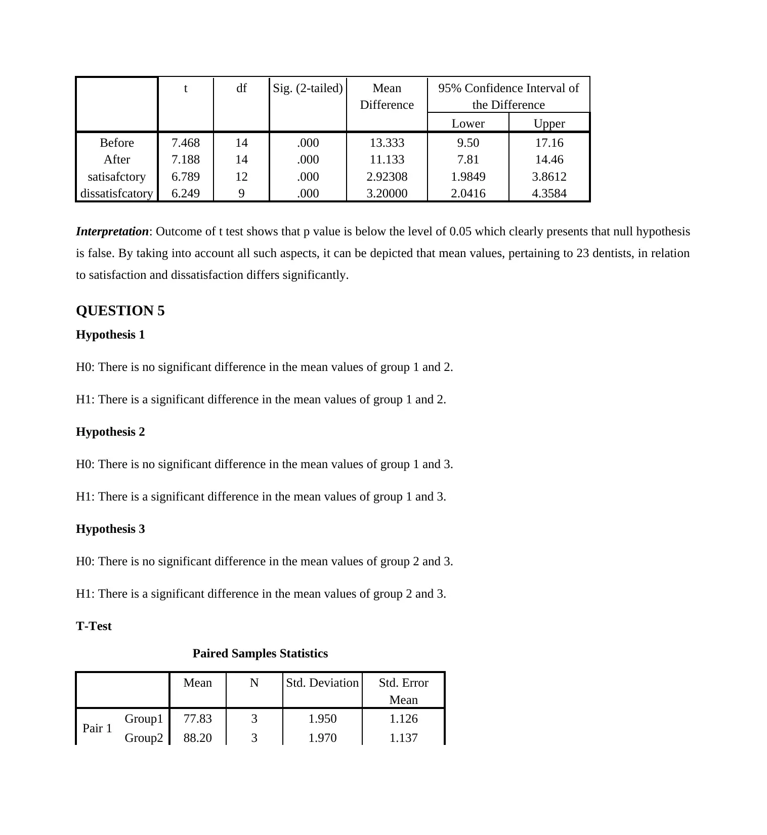
Interpretation: Outcome of t test shows that p value is below the level of 0.05 which clearly presents that null hypothesis
is false. By taking into account all such aspects, it can be depicted that mean values, pertaining to 23 dentists, in relation
to satisfaction and dissatisfaction differs significantly.
QUESTION 5
Hypothesis 1
H0: There is no significant difference in the mean values of group 1 and 2.
H1: There is a significant difference in the mean values of group 1 and 2.
Hypothesis 2
H0: There is no significant difference in the mean values of group 1 and 3.
H1: There is a significant difference in the mean values of group 1 and 3.
Hypothesis 3
H0: There is no significant difference in the mean values of group 2 and 3.
H1: There is a significant difference in the mean values of group 2 and 3.
T-Test
Paired Samples Statistics
Mean N Std. Deviation Std. Error
Mean
Pair 1 Group1 77.83 3 1.950 1.126
Group2 88.20 3 1.970 1.137
Difference
95% Confidence Interval of
the Difference
Lower Upper
Before 7.468 14 .000 13.333 9.50 17.16
After 7.188 14 .000 11.133 7.81 14.46
satisafctory 6.789 12 .000 2.92308 1.9849 3.8612
dissatisfcatory 6.249 9 .000 3.20000 2.0416 4.3584
Interpretation: Outcome of t test shows that p value is below the level of 0.05 which clearly presents that null hypothesis
is false. By taking into account all such aspects, it can be depicted that mean values, pertaining to 23 dentists, in relation
to satisfaction and dissatisfaction differs significantly.
QUESTION 5
Hypothesis 1
H0: There is no significant difference in the mean values of group 1 and 2.
H1: There is a significant difference in the mean values of group 1 and 2.
Hypothesis 2
H0: There is no significant difference in the mean values of group 1 and 3.
H1: There is a significant difference in the mean values of group 1 and 3.
Hypothesis 3
H0: There is no significant difference in the mean values of group 2 and 3.
H1: There is a significant difference in the mean values of group 2 and 3.
T-Test
Paired Samples Statistics
Mean N Std. Deviation Std. Error
Mean
Pair 1 Group1 77.83 3 1.950 1.126
Group2 88.20 3 1.970 1.137
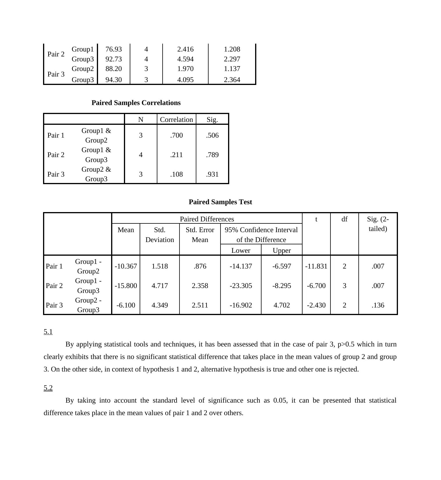
Pair 2 Group1 76.93 4 2.416 1.208
Group3 92.73 4 4.594 2.297
Pair 3 Group2 88.20 3 1.970 1.137
Group3 94.30 3 4.095 2.364
Paired Samples Correlations
N Correlation Sig.
Pair 1 Group1 &
Group2 3 .700 .506
Pair 2 Group1 &
Group3 4 .211 .789
Pair 3 Group2 &
Group3 3 .108 .931
Paired Samples Test
Paired Differences t df Sig. (2-
tailed)Mean Std.
Deviation
Std. Error
Mean
95% Confidence Interval
of the Difference
Lower Upper
Pair 1 Group1 -
Group2 -10.367 1.518 .876 -14.137 -6.597 -11.831 2 .007
Pair 2 Group1 -
Group3 -15.800 4.717 2.358 -23.305 -8.295 -6.700 3 .007
Pair 3 Group2 -
Group3 -6.100 4.349 2.511 -16.902 4.702 -2.430 2 .136
5.1
By applying statistical tools and techniques, it has been assessed that in the case of pair 3, p>0.5 which in turn
clearly exhibits that there is no significant statistical difference that takes place in the mean values of group 2 and group
3. On the other side, in context of hypothesis 1 and 2, alternative hypothesis is true and other one is rejected.
5.2
By taking into account the standard level of significance such as 0.05, it can be presented that statistical
difference takes place in the mean values of pair 1 and 2 over others.
⊘ This is a preview!⊘
Do you want full access?
Subscribe today to unlock all pages.
Trusted by 1+ million students worldwide
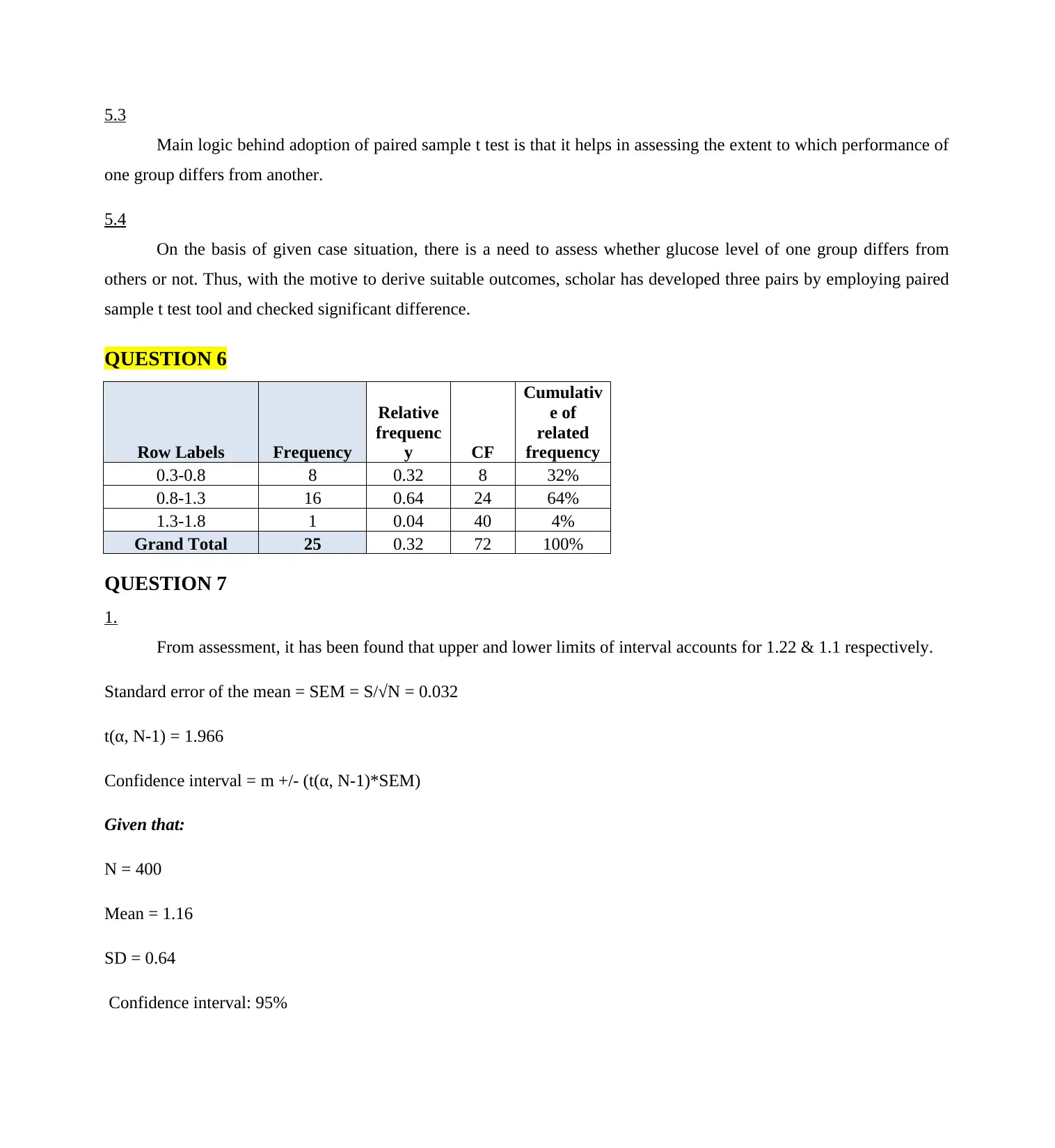
5.3
Main logic behind adoption of paired sample t test is that it helps in assessing the extent to which performance of
one group differs from another.
5.4
On the basis of given case situation, there is a need to assess whether glucose level of one group differs from
others or not. Thus, with the motive to derive suitable outcomes, scholar has developed three pairs by employing paired
sample t test tool and checked significant difference.
QUESTION 6
Row Labels Frequency
Relative
frequenc
y CF
Cumulativ
e of
related
frequency
0.3-0.8 8 0.32 8 32%
0.8-1.3 16 0.64 24 64%
1.3-1.8 1 0.04 40 4%
Grand Total 25 0.32 72 100%
QUESTION 7
1.
From assessment, it has been found that upper and lower limits of interval accounts for 1.22 & 1.1 respectively.
Standard error of the mean = SEM = S/√N = 0.032
t(α, N-1) = 1.966
Confidence interval = m +/- (t(α, N-1)*SEM)
Given that:
N = 400
Mean = 1.16
SD = 0.64
Confidence interval: 95%
Paraphrase This Document
Need a fresh take? Get an instant paraphrase of this document with our AI Paraphraser
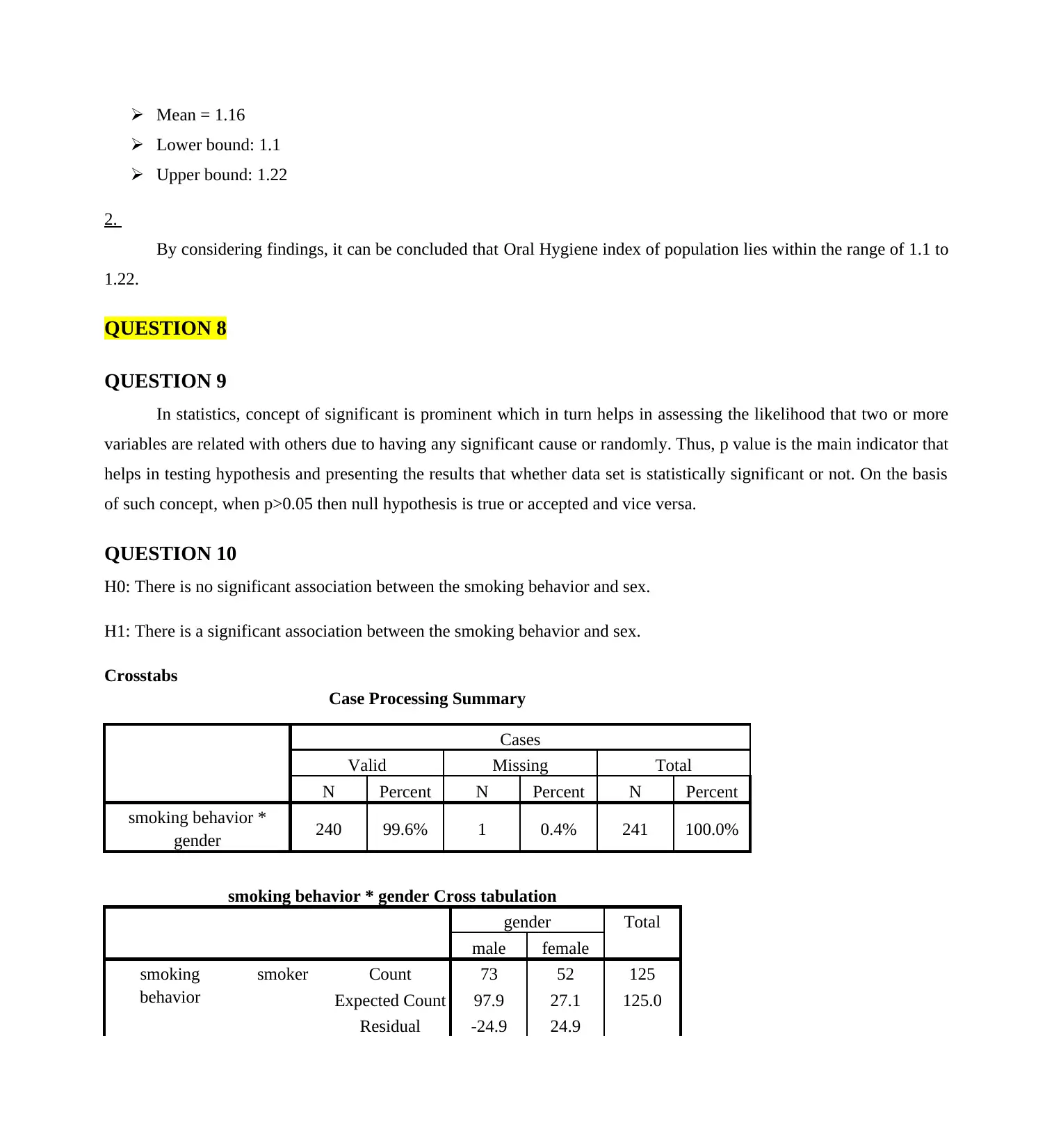
Mean = 1.16
Lower bound: 1.1
Upper bound: 1.22
2.
By considering findings, it can be concluded that Oral Hygiene index of population lies within the range of 1.1 to
1.22.
QUESTION 8
QUESTION 9
In statistics, concept of significant is prominent which in turn helps in assessing the likelihood that two or more
variables are related with others due to having any significant cause or randomly. Thus, p value is the main indicator that
helps in testing hypothesis and presenting the results that whether data set is statistically significant or not. On the basis
of such concept, when p>0.05 then null hypothesis is true or accepted and vice versa.
QUESTION 10
H0: There is no significant association between the smoking behavior and sex.
H1: There is a significant association between the smoking behavior and sex.
Crosstabs
Case Processing Summary
Cases
Valid Missing Total
N Percent N Percent N Percent
smoking behavior *
gender 240 99.6% 1 0.4% 241 100.0%
smoking behavior * gender Cross tabulation
gender Total
male female
smoking
behavior
smoker Count 73 52 125
Expected Count 97.9 27.1 125.0
Residual -24.9 24.9
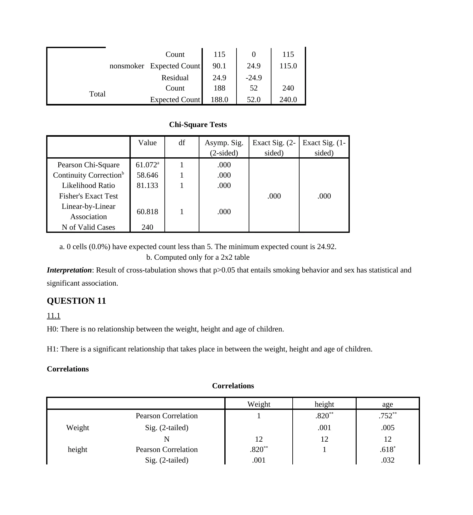
nonsmoker
Count 115 0 115
Expected Count 90.1 24.9 115.0
Residual 24.9 -24.9
Total Count 188 52 240
Expected Count 188.0 52.0 240.0
Chi-Square Tests
Value df Asymp. Sig.
(2-sided)
Exact Sig. (2-
sided)
Exact Sig. (1-
sided)
Pearson Chi-Square 61.072a 1 .000
Continuity Correctionb 58.646 1 .000
Likelihood Ratio 81.133 1 .000
Fisher's Exact Test .000 .000
Linear-by-Linear
Association 60.818 1 .000
N of Valid Cases 240
a. 0 cells (0.0%) have expected count less than 5. The minimum expected count is 24.92.
b. Computed only for a 2x2 table
Interpretation: Result of cross-tabulation shows that p>0.05 that entails smoking behavior and sex has statistical and
significant association.
QUESTION 11
11.1
H0: There is no relationship between the weight, height and age of children.
H1: There is a significant relationship that takes place in between the weight, height and age of children.
Correlations
Correlations
Weight height age
Weight
Pearson Correlation 1 .820** .752**
Sig. (2-tailed) .001 .005
N 12 12 12
height Pearson Correlation .820** 1 .618*
Sig. (2-tailed) .001 .032
⊘ This is a preview!⊘
Do you want full access?
Subscribe today to unlock all pages.
Trusted by 1+ million students worldwide
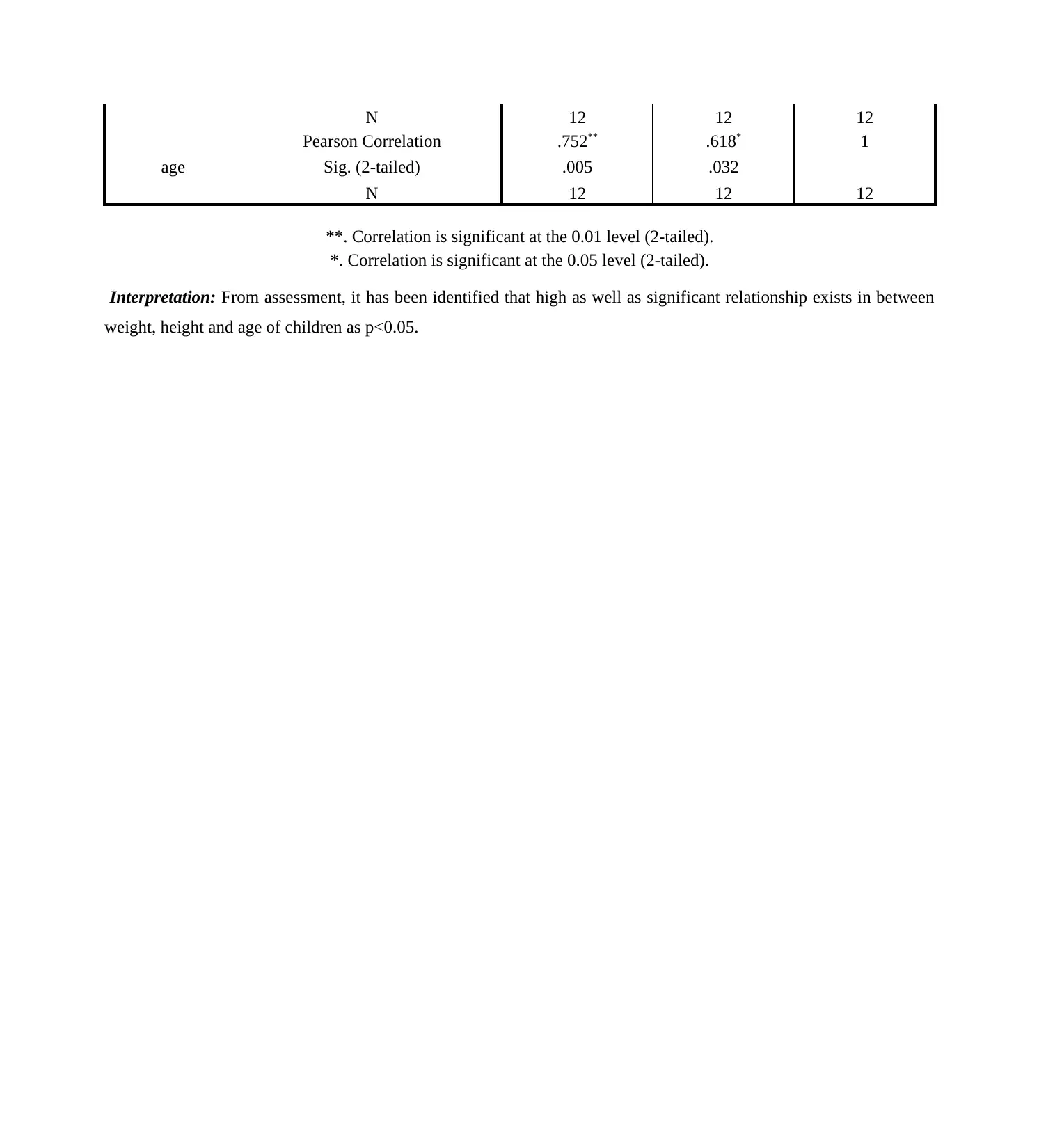
N 12 12 12
age
Pearson Correlation .752** .618* 1
Sig. (2-tailed) .005 .032
N 12 12 12
**. Correlation is significant at the 0.01 level (2-tailed).
*. Correlation is significant at the 0.05 level (2-tailed).
Interpretation: From assessment, it has been identified that high as well as significant relationship exists in between
weight, height and age of children as p<0.05.
Paraphrase This Document
Need a fresh take? Get an instant paraphrase of this document with our AI Paraphraser
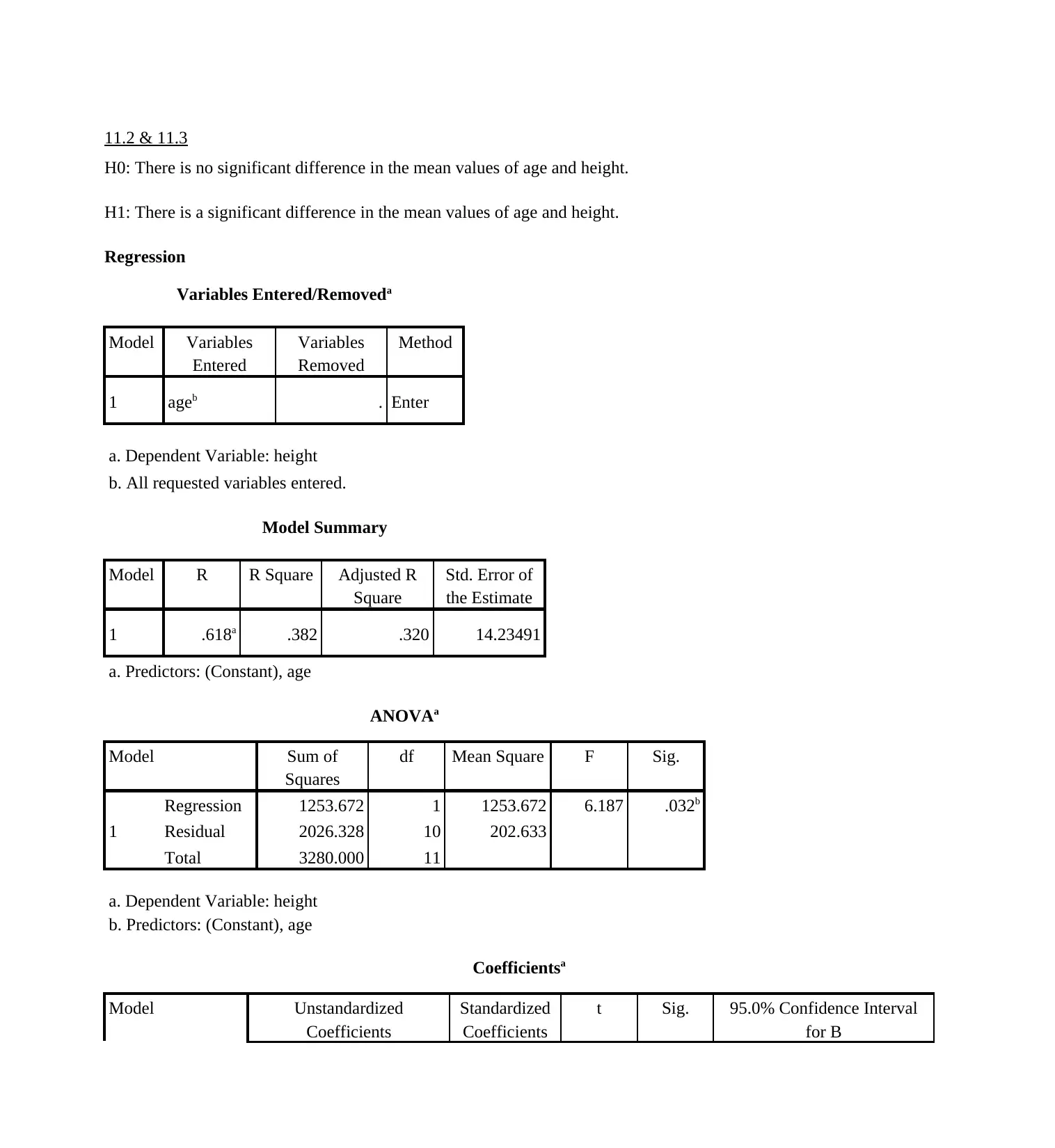
11.2 & 11.3
H0: There is no significant difference in the mean values of age and height.
H1: There is a significant difference in the mean values of age and height.
Regression
Variables Entered/Removeda
Model Variables
Entered
Variables
Removed
Method
1 ageb . Enter
a. Dependent Variable: height
b. All requested variables entered.
Model Summary
Model R R Square Adjusted R
Square
Std. Error of
the Estimate
1 .618a .382 .320 14.23491
a. Predictors: (Constant), age
ANOVAa
Model Sum of
Squares
df Mean Square F Sig.
1
Regression 1253.672 1 1253.672 6.187 .032b
Residual 2026.328 10 202.633
Total 3280.000 11
a. Dependent Variable: height
b. Predictors: (Constant), age
Coefficientsa
Model Unstandardized
Coefficients
Standardized
Coefficients
t Sig. 95.0% Confidence Interval
for B
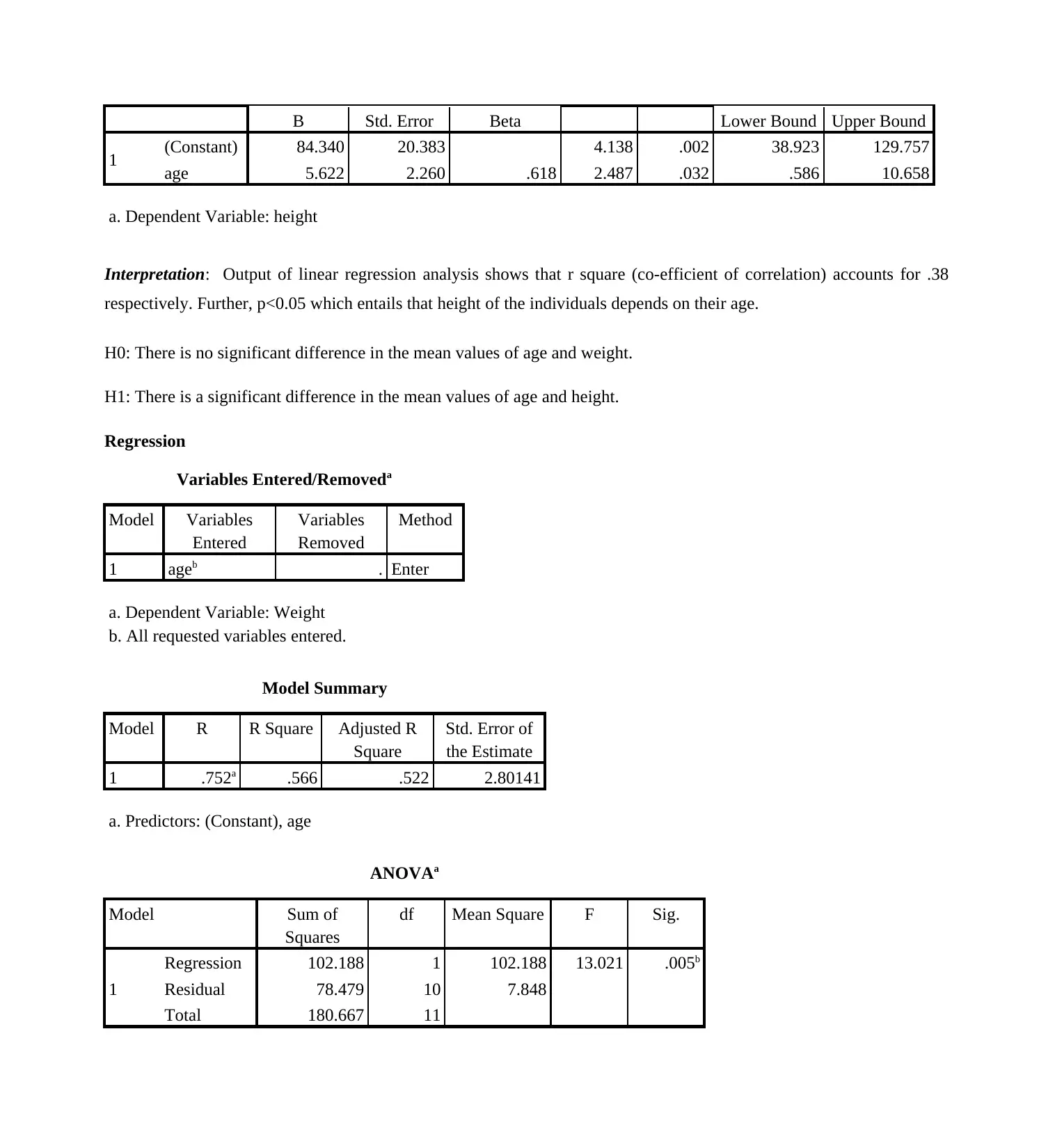
B Std. Error Beta Lower Bound Upper Bound
1 (Constant) 84.340 20.383 4.138 .002 38.923 129.757
age 5.622 2.260 .618 2.487 .032 .586 10.658
a. Dependent Variable: height
Interpretation: Output of linear regression analysis shows that r square (co-efficient of correlation) accounts for .38
respectively. Further, p<0.05 which entails that height of the individuals depends on their age.
H0: There is no significant difference in the mean values of age and weight.
H1: There is a significant difference in the mean values of age and height.
Regression
Variables Entered/Removeda
Model Variables
Entered
Variables
Removed
Method
1 ageb . Enter
a. Dependent Variable: Weight
b. All requested variables entered.
Model Summary
Model R R Square Adjusted R
Square
Std. Error of
the Estimate
1 .752a .566 .522 2.80141
a. Predictors: (Constant), age
ANOVAa
Model Sum of
Squares
df Mean Square F Sig.
1
Regression 102.188 1 102.188 13.021 .005b
Residual 78.479 10 7.848
Total 180.667 11
⊘ This is a preview!⊘
Do you want full access?
Subscribe today to unlock all pages.
Trusted by 1+ million students worldwide
1 out of 13
Related Documents


Your All-in-One AI-Powered Toolkit for Academic Success.
+13062052269
info@desklib.com
Available 24*7 on WhatsApp / Email
![[object Object]](/_next/static/media/star-bottom.7253800d.svg)
Unlock your academic potential
Copyright © 2020–2026 A2Z Services. All Rights Reserved. Developed and managed by ZUCOL.