Industrial Production, Interest Rates, House Prices Analysis

This report presents a comprehensive statistical analysis of three key economic datasets: industrial production, interest rates, and house prices. The analysis begins with the industrial production data, utilizing time series techniques to examine its behavior, including plotting the time series, calculating autocorrelation and partial autocorrelation functions, and testing for stationarity. An ARIMA model is fitted to the data, and its performance is evaluated using the Ljung-Box test. The report then moves on to the interest rate data, employing cointegration tests to examine the relationships between various interest rates. The Johansen procedure is used to determine the number of cointegration relationships, and error correction components are derived. Finally, the report analyzes house price data using a logit model to study the factors influencing home buyer preferences. A full model is fitted, and a stepwise selection process is used to identify an optimal model. The report compares the full and selected models, justifies the choice based on the AIC criteria, and calculates odds and probabilities related to home preferences. The analysis provides insights into the dynamics of these economic variables and offers practical applications of statistical modeling techniques.

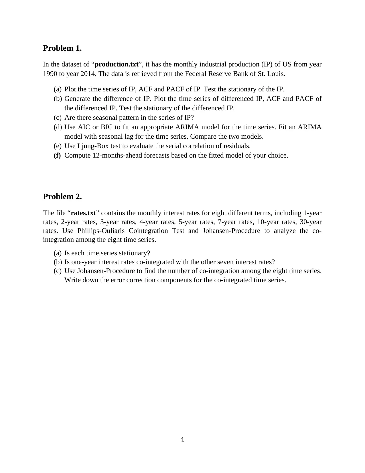
Problem 1.
In the dataset of “production.txt”, it has the monthly industrial production (IP) of US from year
1990 to year 2014. The data is retrieved from the Federal Reserve Bank of St. Louis.
(a) Plot the time series of IP, ACF and PACF of IP. Test the stationary of the IP.
(b) Generate the difference of IP. Plot the time series of differenced IP, ACF and PACF of
the differenced IP. Test the stationary of the differenced IP.
(c) Are there seasonal pattern in the series of IP?
(d) Use AIC or BIC to fit an appropriate ARIMA model for the time series. Fit an ARIMA
model with seasonal lag for the time series. Compare the two models.
(e) Use Ljung-Box test to evaluate the serial correlation of residuals.
(f) Compute 12-months-ahead forecasts based on the fitted model of your choice.
Problem 2.
The file “rates.txt” contains the monthly interest rates for eight different terms, including 1-year
rates, 2-year rates, 3-year rates, 4-year rates, 5-year rates, 7-year rates, 10-year rates, 30-year
rates. Use Phillips-Ouliaris Cointegration Test and Johansen-Procedure to analyze the co-
integration among the eight time series.
(a) Is each time series stationary?
(b) Is one-year interest rates co-integrated with the other seven interest rates?
(c) Use Johansen-Procedure to find the number of co-integration among the eight time series.
Write down the error correction components for the co-integrated time series.
1

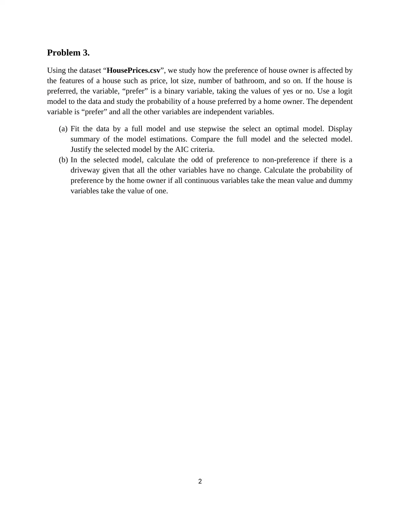
Problem 3.
Using the dataset “HousePrices.csv”, we study how the preference of house owner is affected by
the features of a house such as price, lot size, number of bathroom, and so on. If the house is
preferred, the variable, “prefer” is a binary variable, taking the values of yes or no. Use a logit
model to the data and study the probability of a house preferred by a home owner. The dependent
variable is “prefer” and all the other variables are independent variables.
(a) Fit the data by a full model and use stepwise the select an optimal model. Display
summary of the model estimations. Compare the full model and the selected model.
Justify the selected model by the AIC criteria.
(b) In the selected model, calculate the odd of preference to non-preference if there is a
driveway given that all the other variables have no change. Calculate the probability of
preference by the home owner if all continuous variables take the mean value and dummy
variables take the value of one.
2