Quality Systems Design Assignment: Statistical Analysis and Charts

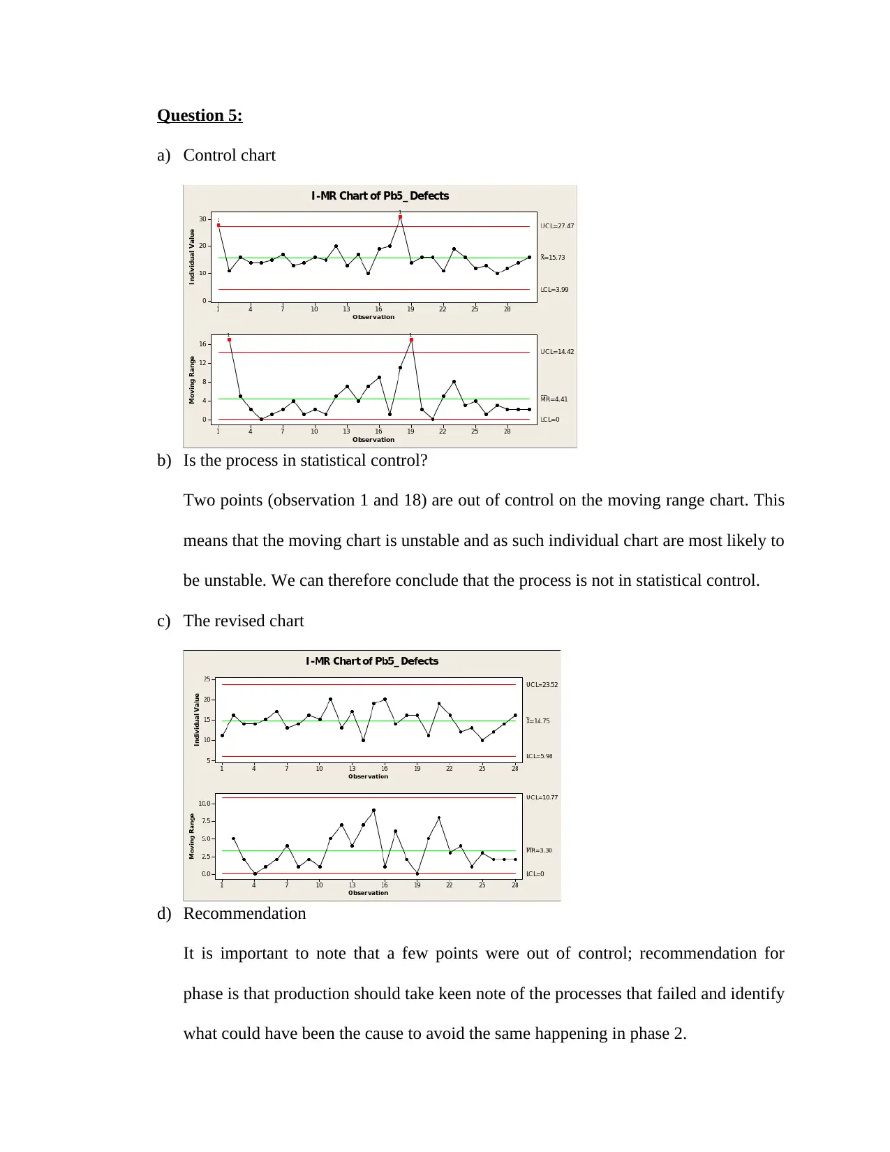
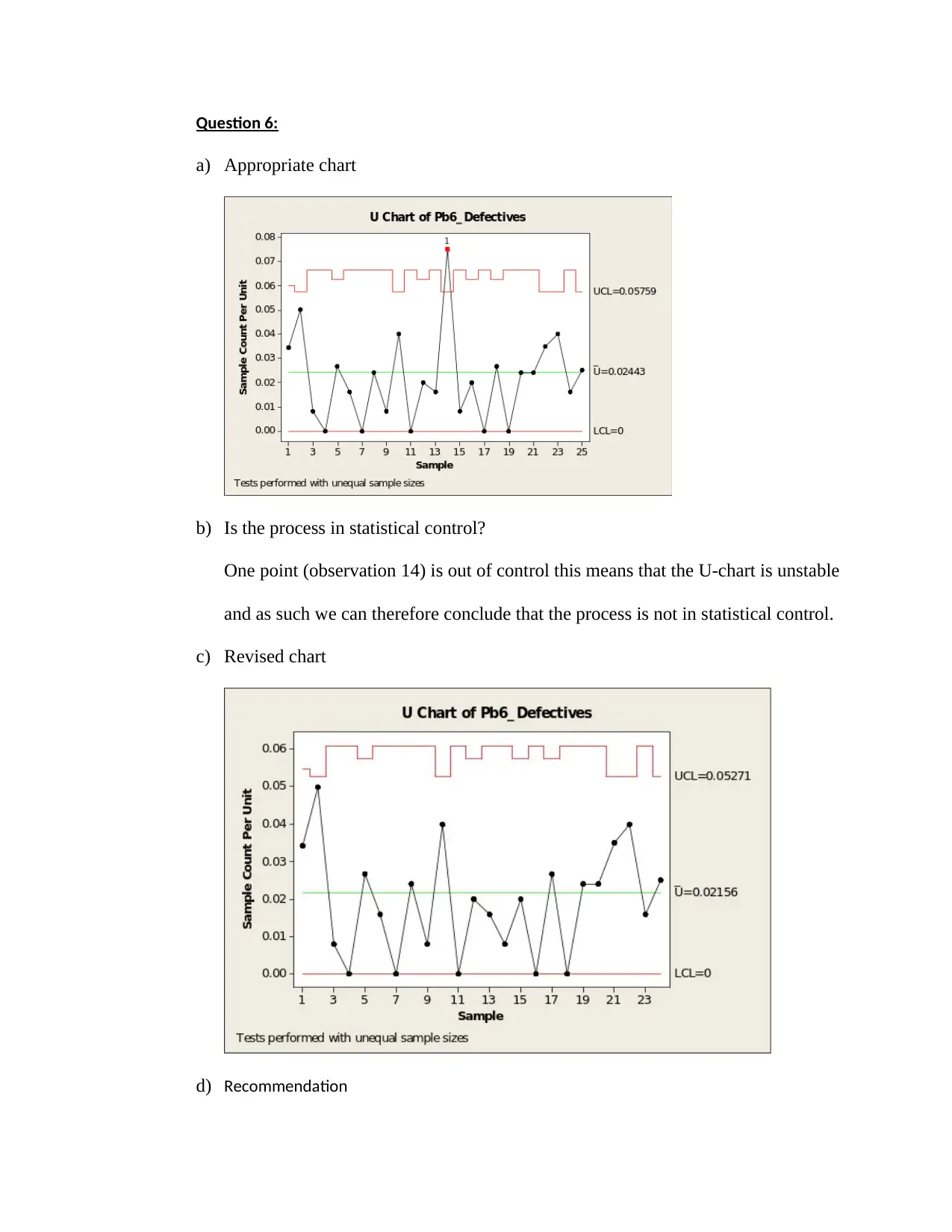
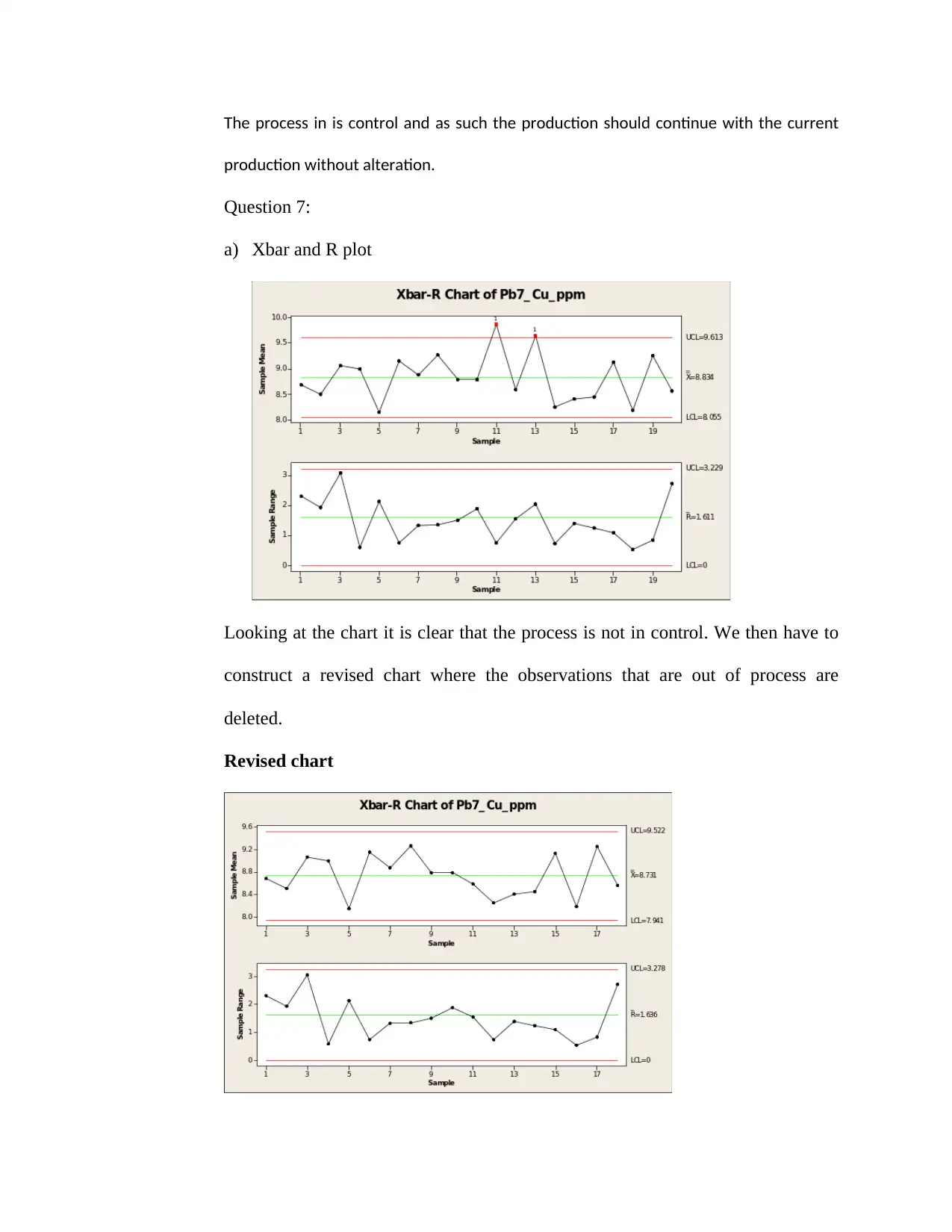
This assignment delves into the statistical analysis of a quality systems design, addressing various questions that require the application of statistical methods and tools. The student begins by analyzing descriptive statistics, including mean, median, and standard deviation, and visualizing data through stem-and-leaf plots and histograms to assess the distribution of data. Hypothesis testing is a central theme, with paired t-tests and ANOVA used to compare means and determine significant differences. The assignment also explores regression analysis to model relationships between variables and assess model adequacy through residual analysis. Control charts, including moving range charts and U-charts, are employed to monitor process stability, identify out-of-control points, and recommend corrective actions. Furthermore, the assignment includes normality testing, process capability analysis, and the application of Cusum and EWMA charts for process monitoring. The design objectives of RL, RL2, and CUSUM are also discussed, providing a comprehensive overview of statistical process control techniques.

Quality Systems Design
Name
University
8th October 2017

Question 1:
a) Answers
Descriptive Statistics: Pb1_Workhours
Variable Mean StDev Minimum Q1 Median Q3 Maximum
Pb1_Workhours 122.18 15.89 97.00 111.00 120.00 132.25 162.00
The above results shows that the mean is 122.18 while the median is 120. The standard
deviation is 15.89. The values shows that the data is close to normally being distributed.
We can therefore say that the data is normally distributed.
b) Answer
The stem and leaf plot below;
Stem-and-leaf plot (Pb1_Workhours):
Unit: 10
9 7 8 8
10 0 0 3 5 7 8 9 9
11 1 1 2 2 2 3 3 4 6 6 7 8 9
12 0 0 2 2 4 4 4 8 8 8
13 1 1 1 2 3 3 5 6 8 8
14 2 6
15 0 5 8
16 2
The shape and distribution of the stem-and-leaf plot shows that the data is normally
distributed.
c) Answer
Histogram

The histogram above suggest that the data is normally distributed
d) Answers
Probability plot

Question 2:
a) Hypothesis
The hypothesis for the given test is;
H0 : μA =μB
H A : μA ≠ μB
That is;
H0: The before is the same as the mean after
HA: The before is not the same as the mean after
b) Interpretation of the p-value;
Paired T-Test and CI: Pb2_Before, Pb2_After
Paired T for Pb2_Before - Pb2_After
N Mean StDev SE Mean
Pb2_Before 10 5.03200 0.58309 0.18439
Pb2_After 10 5.52600 0.44257 0.13995
Difference 10 -0.494000 0.881542 0.278768
95% CI for mean difference: (-1.124617, 0.136617)
T-Test of mean difference = 0 (vs not = 0): T-Value = -1.77 P-Value = 0.110
The p-value is given as 0.110 (a value greater than 5% level of significance0, we
therefore fail to reject the null hypothesis and conclude that the mean completion
times before and after are not significantly different.

Question 3:
a) Hypothesis
The hypothesis tested for this question is;
H0 : μ1=μ2=μ3
H A : At least one of the meansis different
One-way ANOVA: Pb3_WearTime versus Pb3_Formula
Source DF SS MS F P
Pb3_Formula 2 17093 8547 22.99 0.000
Error 27 10039 372
Total 29 27133
S = 19.28 R-Sq = 63.00% R-Sq(adj) = 60.26%
Individual 95% CIs For Mean Based on
Pooled StDev
Level N Mean StDev -+---------+---------+---------+--------
1 10 284.90 15.28 (----*----)
2 10 320.90 13.30 (----*----)
3 10 342.80 26.55 (----*----)
-+---------+---------+---------+--------
275 300 325 350
Pooled StDev = 19.28

b) Plot and analysis of residuals
We sought to analyze the residual by checking whether the residuals follow a normal
distribution. The normal plot is given below;
The above normal plot shows that the data is normally distributed. This therefore
means the necessary assumption of normality has been met.
c) The formulation with the highest mean wear time;
From the above analysis, it is evident that formulation 3 has the highest mean wear
time (M = 342.80, SD = 26.55) as compared to the other two.

Question 4:
a) Hypothesis of the question
The hypothesis to be tested for this question is;
H0: β1 = β2 = β3 = 0
H1: At least one β is not zero
Regression results;
Regression Analysis: Pb4_Volume versus Pb4_Diameter, Pb4_Length, .
The regression equation is
Pb4_Volume = - 36.3 + 30.5 Pb4_Diameter + 4.77 Pb4_Length + 1.25 Pb4_Cycles
Predictor Coef SE Coef T P
Constant -36.2579 0.4677 -77.52 0.000
Pb4_Diameter 30.4946 0.5778 52.77 0.000
Pb4_Length 4.76576 0.00922 516.84 0.000
Pb4_Cycles 1.25134 0.01009 124.04 0.000
S = 0.00841452 R-Sq = 100.0% R-Sq(adj) = 100.0%
Analysis of Variance
Source DF SS MS F P
Regression 3 19.8206 6.6069 93311.67 0.000
Residual Error 29 0.0021 0.0001
Total 32 19.8226
Source DF Seq SS
Pb4_Diameter 1 0.7936
Pb4_Length 1 17.9376
Pb4_Cycles 1 1.0894
Unusual Observations
Obs Pb4_Diameter Pb4_Volume Fit SE Fit Residual St Resid
5 0.799 10.6639 10.6443 0.0039 0.0196 2.62R
6 0.791 12.4260 12.4243 0.0054 0.0017 0.26 X
17 0.796 10.2603 10.2819 0.0040 -0.0216 -2.93R
22 0.796 11.1412 11.1264 0.0046 0.0148 2.11R
30 0.801 12.8889 12.8726 0.0029 0.0163 2.06R
R denotes an observation with a large standardized residual.
X denotes an observation whose X value gives it large influence.

b) Analyzing residuals
The plots below are meant to check the model adequacy;
i) Normality check
The normal plot above shows that the residuals are not normally
distributed
ii) Constant variance check
The points on the above plot appears to be randomly scattered around zero, so the
assumption that the error terms have a mean of zero is reasonable. Also, looking at the
vertical width of the scatter, it appears not to decrease or increase across the fitted values,
with that we can make an assumption that the variance in the error terms is constant.

Question 5:
a) Control chart
b) Is the process in statistical control?
Two points (observation 1 and 18) are out of control on the moving range chart. This
means that the moving chart is unstable and as such individual chart are most likely to
be unstable. We can therefore conclude that the process is not in statistical control.
c) The revised chart
d) Recommendation
It is important to note that a few points were out of control; recommendation for
phase is that production should take keen note of the processes that failed and identify
what could have been the cause to avoid the same happening in phase 2.

Question 6:
a) Appropriate chart
b) Is the process in statistical control?
One point (observation 14) is out of control this means that the U-chart is unstable
and as such we can therefore conclude that the process is not in statistical control.
c) Revised chart
d) Recommendation

The process in is control and as such the production should continue with the current
production without alteration.
Question 7:
a) Xbar and R plot
Looking at the chart it is clear that the process is not in control. We then have to
construct a revised chart where the observations that are out of process are
deleted.
Revised chart

b) Mean and standard deviation of the revised process is;
Descriptive Statistics: Pb7_Cu_ppm
Variable N N* Mean StDev
Pb7_Cu_ppm 108 0 8.7311 0.6888
The mean is 8.7311 while the standard deviation is 0.6888.
c) Is the layer thickness revised normally distributed?
Yes it is normally distributed; as can be seen, the plot is almost linear and also the p-
value of Anderson-Darling (AD) is 0.199 (a value greater than 5% level of
significance), we fail to reject the null hypothesis of normality and conclude that the
data is normally distributed.
d) Capability process
C p= USL−LSL
6∗stdev
Specifications are 9.0 ± 1.50 ppm
USL = 9.0 + 1.50 = 10.50
LSL = 9.0 - 1.50 = 7.50