Statistical Analysis of Credit Card Spending and Family Size

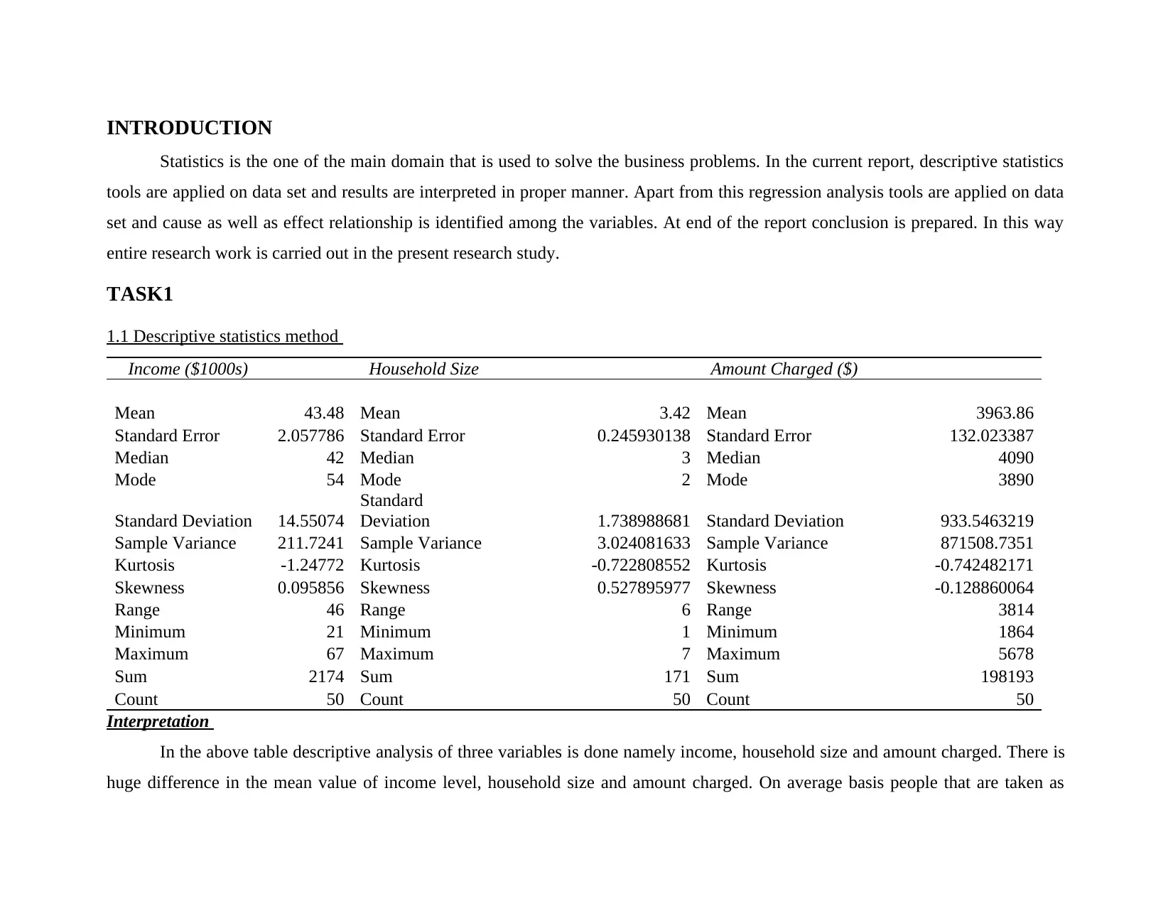
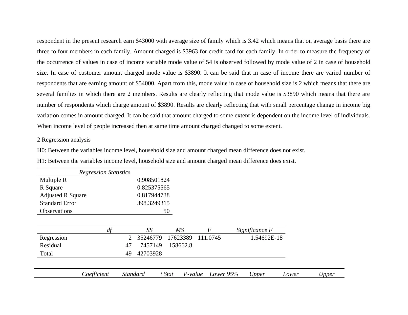
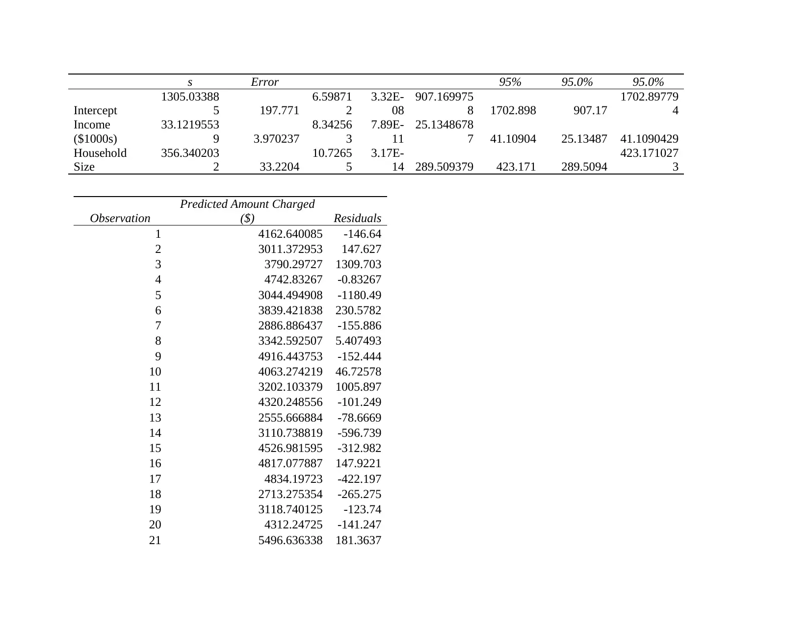
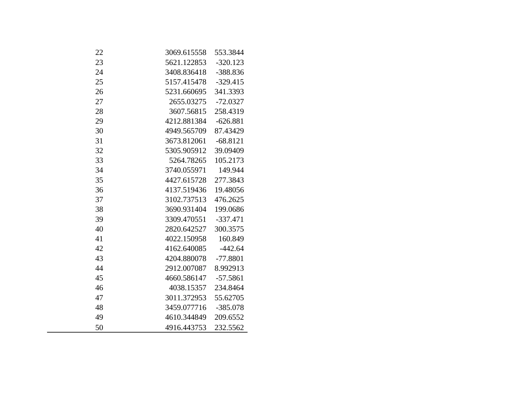
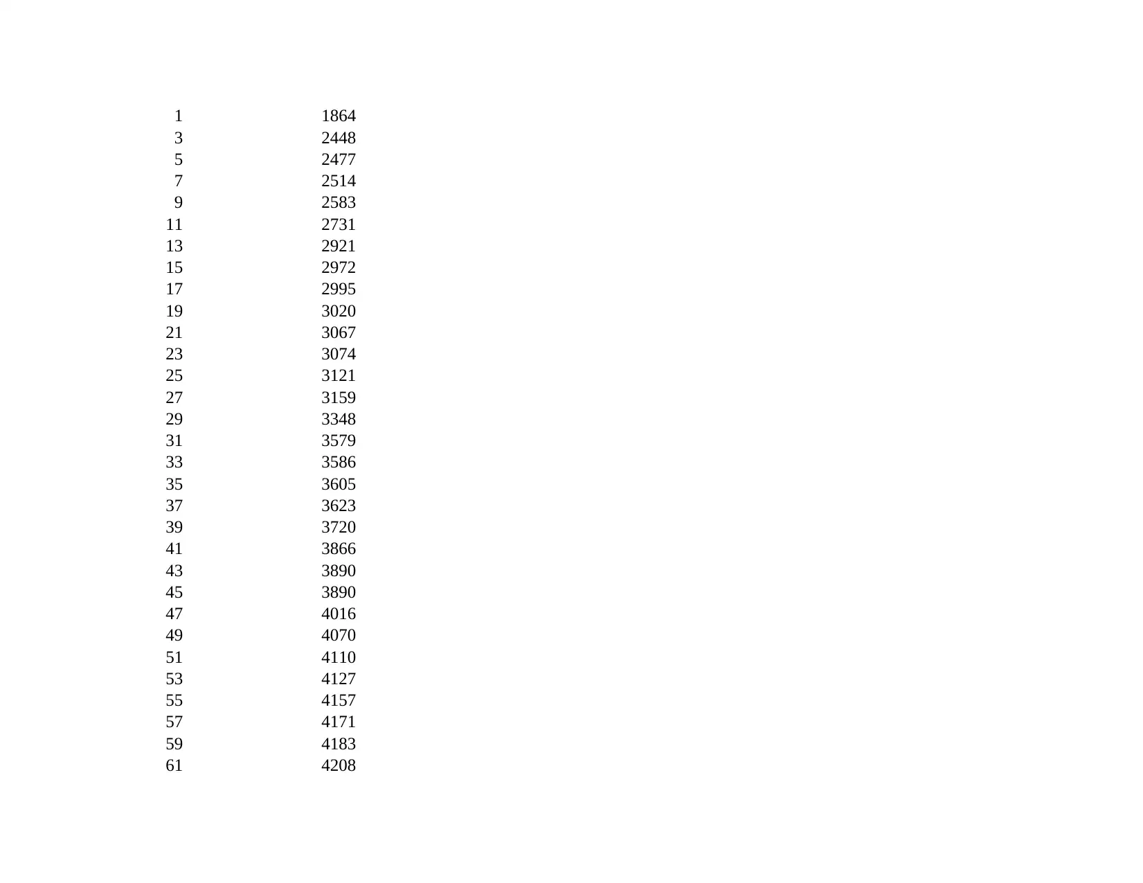
This report presents a comprehensive statistical analysis of credit card spending, household size, and income levels. The study begins with descriptive statistics, providing an overview of the mean, median, mode, and standard deviation for each variable. Regression analysis is then employed to identify the relationships between these variables, with a focus on how income and family size impact credit card charges. The report includes regression equations, interpretations of the results, and the addition of variables to refine the model. Further analysis includes histograms, descriptive statistics, and correlation analysis of exam and assignment scores. Finally, ANOVA is used to assess depression levels across different cities, with a discussion on the appropriateness of treatment methods. The findings provide valuable insights into consumer behavior and statistical methodologies.

STATISTICS AND RESEARCH

TABLE OF CONTENTS
INTRODUCTION.......................................................................................................................................................................................3
TASK1.........................................................................................................................................................................................................3
1.1 Descriptive statistics method.............................................................................................................................................................3
2 Regression analysis...............................................................................................................................................................................4
3 Regression equation............................................................................................................................................................................11
4 Family size and credit card change in expenses.................................................................................................................................11
5 Addition of variable to model.............................................................................................................................................................12
TASK 2......................................................................................................................................................................................................12
Activity 01.............................................................................................................................................................................................12
Activity 02.............................................................................................................................................................................................12
Activity 03.............................................................................................................................................................................................24
TASK 3......................................................................................................................................................................................................26
1 Descriptive statistics...........................................................................................................................................................................26
2 ANNOVA...........................................................................................................................................................................................27
3 Appropriateness of treatment..............................................................................................................................................................29
CONCLUSION..........................................................................................................................................................................................29

INTRODUCTION
Statistics is the one of the main domain that is used to solve the business problems. In the current report, descriptive statistics
tools are applied on data set and results are interpreted in proper manner. Apart from this regression analysis tools are applied on data
set and cause as well as effect relationship is identified among the variables. At end of the report conclusion is prepared. In this way
entire research work is carried out in the present research study.
TASK1
1.1 Descriptive statistics method
Income ($1000s) Household Size Amount Charged ($)
Mean 43.48 Mean 3.42 Mean 3963.86
Standard Error 2.057786 Standard Error 0.245930138 Standard Error 132.023387
Median 42 Median 3 Median 4090
Mode 54 Mode 2 Mode 3890
Standard Deviation 14.55074
Standard
Deviation 1.738988681 Standard Deviation 933.5463219
Sample Variance 211.7241 Sample Variance 3.024081633 Sample Variance 871508.7351
Kurtosis -1.24772 Kurtosis -0.722808552 Kurtosis -0.742482171
Skewness 0.095856 Skewness 0.527895977 Skewness -0.128860064
Range 46 Range 6 Range 3814
Minimum 21 Minimum 1 Minimum 1864
Maximum 67 Maximum 7 Maximum 5678
Sum 2174 Sum 171 Sum 198193
Count 50 Count 50 Count 50
Interpretation
In the above table descriptive analysis of three variables is done namely income, household size and amount charged. There is
huge difference in the mean value of income level, household size and amount charged. On average basis people that are taken as

respondent in the present research earn $43000 with average size of family which is 3.42 which means that on average basis there are
three to four members in each family. Amount charged is $3963 for credit card for each family. In order to measure the frequency of
the occurrence of values in case of income variable mode value of 54 is observed followed by mode value of 2 in case of household
size. In case of customer amount charged mode value is $3890. It can be said that in case of income there are varied number of
respondents that are earning amount of $54000. Apart from this, mode value in case of household size is 2 which means that there are
several families in which there are 2 members. Results are clearly reflecting that mode value is $3890 which means that there are
number of respondents which charge amount of $3890. Results are clearly reflecting that with small percentage change in income big
variation comes in amount charged. It can be said that amount charged to some extent is dependent on the income level of individuals.
When income level of people increased then at same time amount charged changed to some extent.
2 Regression analysis
H0: Between the variables income level, household size and amount charged mean difference does not exist.
H1: Between the variables income level, household size and amount charged mean difference does exist.
Regression Statistics
Multiple R 0.908501824
R Square 0.825375565
Adjusted R Square 0.817944738
Standard Error 398.3249315
Observations 50
df SS MS F Significance F
Regression 2 35246779 17623389 111.0745 1.54692E-18
Residual 47 7457149 158662.8
Total 49 42703928
Coefficient Standard t Stat P-value Lower 95% Upper Lower Upper

s Error 95% 95.0% 95.0%
Intercept
1305.03388
5 197.771
6.59871
2
3.32E-
08
907.169975
8 1702.898 907.17
1702.89779
4
Income
($1000s)
33.1219553
9 3.970237
8.34256
3
7.89E-
11
25.1348678
7 41.10904 25.13487 41.1090429
Household
Size
356.340203
2 33.2204
10.7265
5
3.17E-
14 289.509379 423.171 289.5094
423.171027
3
Observation
Predicted Amount Charged
($) Residuals
1 4162.640085 -146.64
2 3011.372953 147.627
3 3790.29727 1309.703
4 4742.83267 -0.83267
5 3044.494908 -1180.49
6 3839.421838 230.5782
7 2886.886437 -155.886
8 3342.592507 5.407493
9 4916.443753 -152.444
10 4063.274219 46.72578
11 3202.103379 1005.897
12 4320.248556 -101.249
13 2555.666884 -78.6669
14 3110.738819 -596.739
15 4526.981595 -312.982
16 4817.077887 147.9221
17 4834.19723 -422.197
18 2713.275354 -265.275
19 3118.740125 -123.74
20 4312.24725 -141.247
21 5496.636338 181.3637

22 3069.615558 553.3844
23 5621.122853 -320.123
24 3408.836418 -388.836
25 5157.415478 -329.415
26 5231.660695 341.3393
27 2655.03275 -72.0327
28 3607.56815 258.4319
29 4212.881384 -626.881
30 4949.565709 87.43429
31 3673.812061 -68.8121
32 5305.905912 39.09409
33 5264.78265 105.2173
34 3740.055971 149.944
35 4427.615728 277.3843
36 4137.519436 19.48056
37 3102.737513 476.2625
38 3690.931404 199.0686
39 3309.470551 -337.471
40 2820.642527 300.3575
41 4022.150958 160.849
42 4162.640085 -442.64
43 4204.880078 -77.8801
44 2912.007087 8.992913
45 4660.586147 -57.5861
46 4038.15357 234.8464
47 3011.372953 55.62705
48 3459.077716 -385.078
49 4610.344849 209.6552
50 4916.443753 232.5562

Percentile Amount Charged ($)

1 1864
3 2448
5 2477
7 2514
9 2583
11 2731
13 2921
15 2972
17 2995
19 3020
21 3067
23 3074
25 3121
27 3159
29 3348
31 3579
33 3586
35 3605
37 3623
39 3720
41 3866
43 3890
45 3890
47 4016
49 4070
51 4110
53 4127
55 4157
57 4171
59 4183
61 4208

63 4214
65 4219
67 4273
69 4412
71 4603
73 4705
75 4742
77 4764
79 4820
81 4828
83 4965
85 5037
87 5100
89 5149
91 5301
93 5345
95 5370
97 5573
99 5678

Figure 1Income residual chart
Figure 2Household size chart

Figure 3Income line fit plot
Figure 4Household size line fit plot
Interpretation
Results are clearly reflecting that there is no significant mean difference between variables household size, income level and
amount charged on credit card. This fact is supported by the fact that level of significance value is 1.50>0.05. This means that there is
no big difference in the rate of change that is happening in average amount customer charged and household size as well as income

level. From the model it can be observed that value of multiple R is 0.90 and same of R square is 0.82. These results are clearly
indicating that there is high value of correlation which is 0.90 which means that with change in relevant independent variable big
variation comes in the dependent variable. Results are clearly reflecting that with change in relevant variable 82% variation comes in
the credit card charge. Intercept value is $1305 which means that even independent variable value is zero average amount charged on
credit card is equal to the mentioned value. Beta value is 33.12 for income level and this reflects that in case slight variation comes in
income level credit card charge amount will change by 33.12 points. On other hand, if household size will change then in that case
average spend on credit card will change by 356 points.
3 Regression equation
Income level and household size are the two variables on which regression equation is prepared above. In the equation income level
intercept value is 1305 beta value of income level for credit card spending is 33.12. In same way for household size intercept value is
1305 and beta value is 356 for same variable in respect to spending on credit card. By putting values in X prediction for customer
spend on credit card can be made.
4 Family size and credit card change in expenses
Household size= a+ bx
= 1305+356*3=2373
If people income level will be $40000 and family size will be three then in that case dependent variable value will be $2373.

5 Addition of variable to model
Apart from the variables that are already included in the model household saving rate is the another one that can be considered
in the model to identify significant relationship between the variables.
TASK 2
Activity 01
Data are arranged in variable view in excel sheet.
Activity 02
(a)Drawing histogram

(b)Descriptive statistics
Student
ID Year
Enrolled
HI001
FINAL
EXAM
HI001
ASSIGNMEN
T 01
HI001
ASSIGNMEN
T 02
HI002
FINAL
EXAM
HI002
ASSIGNMEN
T 01
HI002
ASSIGNMEN
T 02
HI003
FINAL
EXAM
Mean 2013.04 32.39 17.21 15.46 26.77 17.82 12.42 25.99
STDEV 0.81124
4.99551
3 1.990959 2.31164
5.28264
7 3.44125 1.989267
8.27179
4
MIN 2012.00 20.00 8.00 8.00 12.00 4.00 4.00 4.00
MAX 2014.00 45.00 22.00 21.00 40.00 22.00 16.00 43.00
18.19 13.54 49.50
3.907851 1.759618 28.43413442
10.00 8.00 1.00
30.00 20.00 98.00
Interpretation
Results are clearly reflecting that HI001 final exam mean value is 32.39 and same for HI002 final exam is 7.82 followed by
HI003 final exam whose mean value is 25.99. It can be seen that standard deviation is high in case of HI003 final exam then HI002
and HI001 final exam. It can be said that in HI003 less marks are gained and also same deviate at fast rate. Means that students earn
marks at different rate and performance in the relevant subject is not good. In case other assignment exams of HI001, HI002 and
HI003 same trend is observed.

Activity 03

Interpretation

 HI001 final exam: Value of level of significance in case of HI001 and HI003 2 assignments is 0.01 and 0.03<0.05. In case of
HI002 1st test and HI003 correlation value is in minus. With some variables HI001 final exam have positive and negative
relationship.
 H1001 assignment 01: Positive correlation is observed in case of HI001 assignments and HI003 final exam. Negative value of
observed in case of HI002 final exam and 1st assignment which are -0.15 and -0.97.
 HI001 assignment 02: HI001 assignment have positive relationship with HI003 final exam and HI003 assignment1. Inverse
relationship is observed in case of HI001 assignment 02.
 HI002 final exam: P value is for HI003 final exam 0.116(0.257>0.05). There is moderate relationship among both variables.
 HI002 assignment 01: Significance value is 0.549(0.00>0.05) for 2nd assignment of HI002 and 0.016(0.880>0.05) for HI003
final exam. Inverse association is observed in case of first assignment of HI003. This line is supported by the fact -
232(0.02<0.05).
 HI002 assignment 02: On analysis of facts it can be identified that 2nd assignment of HI002 is positively related final exam of
HI003. Mentioned variable is inversely related with first assignment of HI003 -.192(0.05=0.05). Similar thing is find out in
respect to HI003.
 HI003 final exam: Results are indicating that final exam is positively related to assignment 1 and assignment 2.
 HI003 assignment 01: There is positive relationship between first and second assignment 0.520 (0.00<0.05). It can be said
that both are interrelated to each other.
TASK 3
1 Descriptive statistics

Interpretation
Results are clearly indicating that depression level is high in case of North Carolina if individuals that are taken as sample units
are healthy in nature. Standard deviation is 6 in case of Florida, 8 in case of New York and 7.5 in case of North Carolina. Standard
deviation value increased at rapid rate in all these cities when respondents taken are suffered from specific disease. Thus, rate of
change in depression level is different for all these cities when individual is or not suffered from depression.
2 ANNOVA

H0: There is no significant mean difference in depression level across studied cities when people are healthy.
HI: There is significant mean difference in depression level across studied cities when people are healthy
Interpretation
Level of significance is 0.008<0.05 which means that depression level is different across cities when individual is healthy. This
fact is clearly reflected by difference that is between mean values of mentioned cities.
H0: There is no significant mean difference in depression level across studied cities when people are not healthy.
HI: There is significant mean difference in depression level across studied cities when people are not healthy.
Interpretation
Level of significance value is 0.49>0.05 and this reflects that there is no significant difference in mean value of depression
across different cities. Fact is supported by similar mean value that is observed in case of different cities.

3 Appropriateness of treatment
Meditation can be done by the individuals that are facing lots of stress in their life. By doing so problem can be solved to some
extent.
CONCLUSION
On the basis of above discussion it is concluded that there is significant importance of statistics for the managers of the
business firms. This is because by using same relationship between different variables is identified in proper manner and managers
quickly make business decisions. It is concluded that level of depression in human body to some extent depends on health and city. If
one is healthy them level of depression is different across cities. Moreover, if one is unhealthy then in that case depression level of
same level is observed.