Public Health: Statistical Analysis of Healthy Lifestyle Data Report

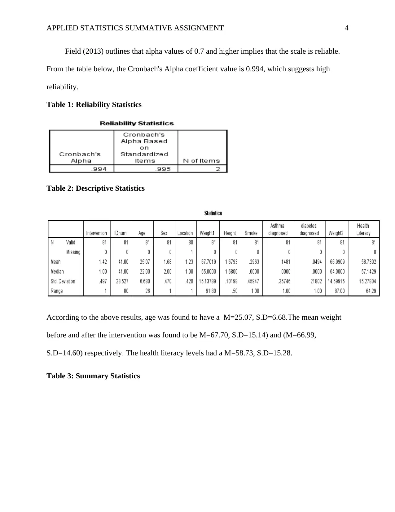
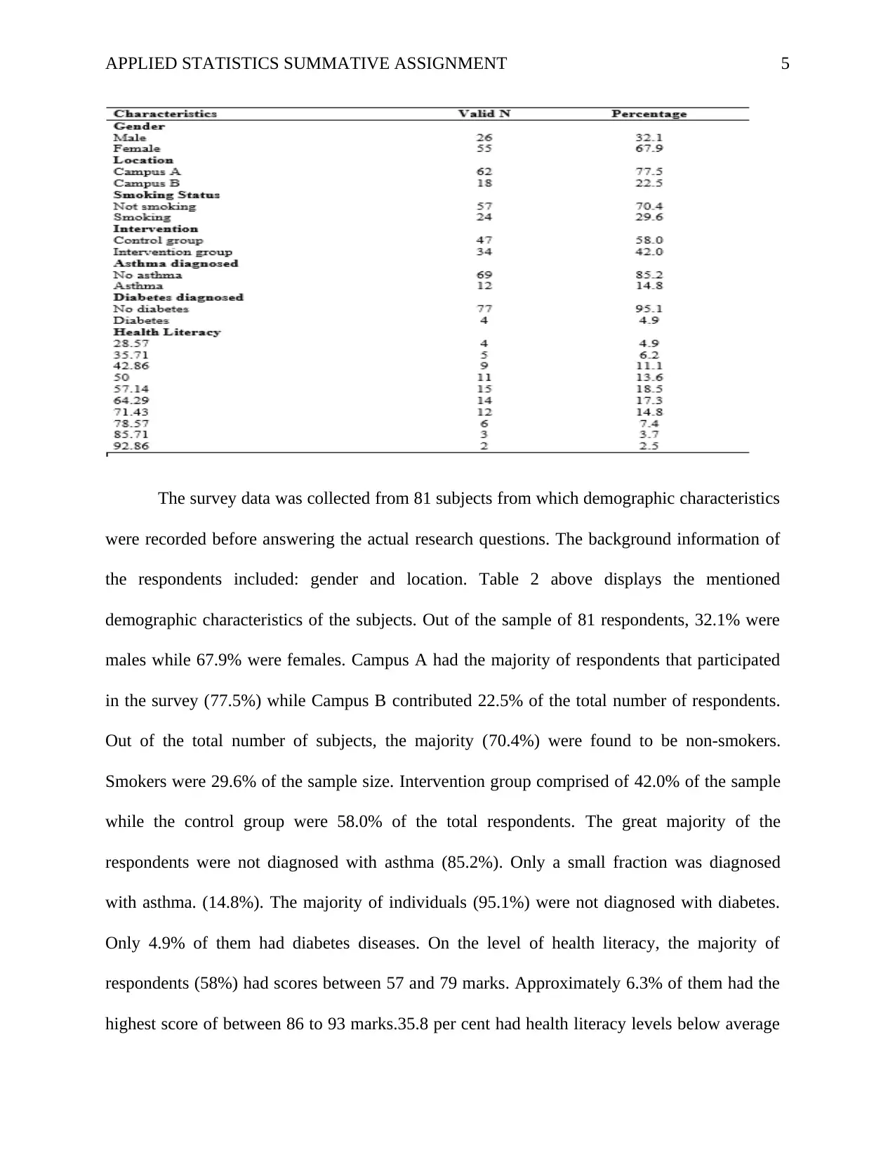
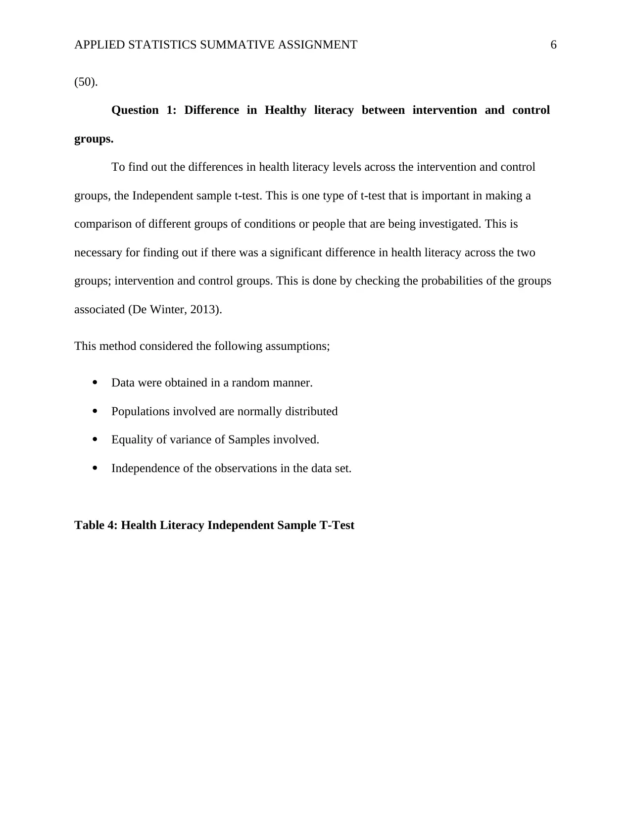
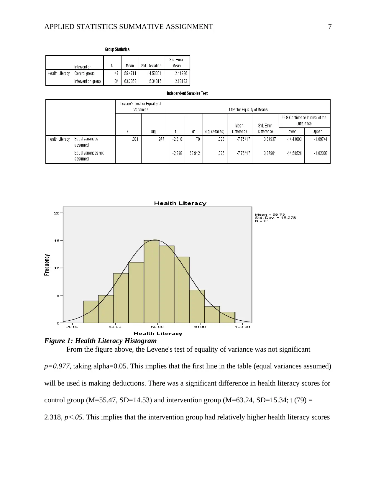
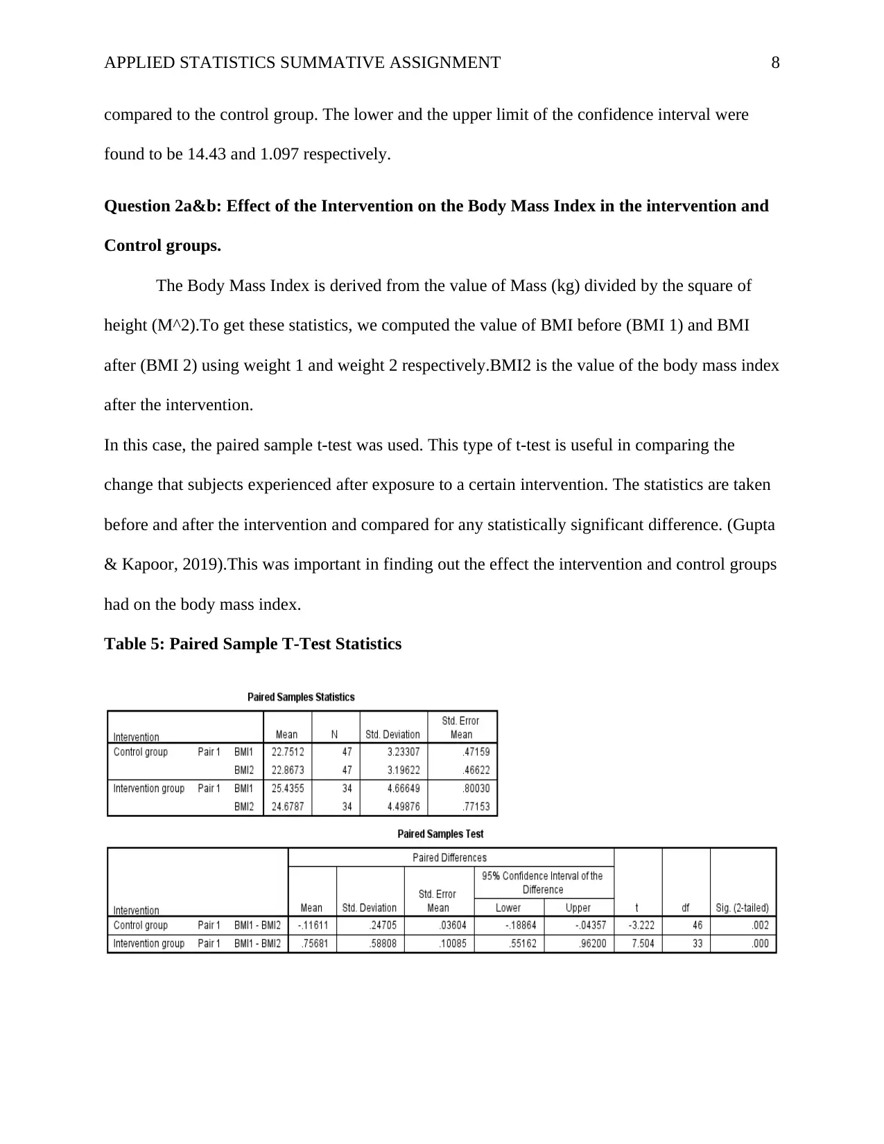
This report presents a statistical analysis of a healthy lifestyle intervention aimed at university students, focusing on improving health literacy and reducing weight. The study involved 81 participants, divided into intervention and control groups, with data collected on age, gender, height, smoking status, health literacy, and health conditions. The analysis employed both descriptive and inferential statistics, using SPSS software. Reliability was assessed using Cronbach's Alpha, demonstrating high internal consistency. Key findings include significant differences in health literacy between the intervention and control groups, with the intervention group showing higher scores. Additionally, the intervention group exhibited a significant reduction in BMI, indicating a positive impact on weight management. The report also explores the effects of the intervention on BMI compared to the control group, as well as the diabetes risk between the two groups, utilizing t-tests, Mann-Whitney U Test and Chi-square tests. Finally, the report investigates the predictive power of health literacy, age, and sex on changes in BMI. The report provides detailed statistical results, including tables and figures, to support the conclusions drawn regarding the effectiveness of the intervention.

Running head: APPLIED STATISTICS SUMMATIVE ASSIGNMENT
1
Healthy Life Style Data Analysis
Student’s Name
Institutional Affiliation

APPLIED STATISTICS SUMMATIVE ASSIGNMENT 2
Healthy Life Style Data Analysis
Background
Statistics is a branch of mathematics that deals with data collection, data classification,
data analysis, and its interpretation to make viable conclusions. It is divided into descriptive and
inferential statistics. Descriptive statistics gives the general summaries and patterns in a dataset
while inferential statistics is concerned with in-depth analysis of data (Gupta & Kapoor, 2019).
Statistics is highly used in many sectors in any economy for planning and decision making. One
of the many sectors it is used is public health. It is necessarily used in as an assessment function.
The government through the ministry of health is able to identify risks, threats, prepare budgets
and make the planning of programs to be carried out. One of the central parts of public health is
the population. Statistics, therefore, will give incites on how to study the population and interpret
data. This involves numbers that describe the population and the science of analyzing concepts
from the population. In general, statistics form part of the vital signs in the field of public health.
The government needs to collect data of its population from birth (birth certificate issued) to
dying of a citizen. A periodic census is also carried out. In health statistics, this information can
be used to compute birth rate, death rates, the fertility rate among others. Health statistics are
vital in providing insight for health policies, identification of problems in the population,
administrative decision making (Bailey,1977).Program planning among others. This will
eventually lead to the provision of better health.
In this study, a random sample of individuals was taken and included in the collection of
data for public health analysis and report. The sample consisted of 81 individuals. The
individuals were informed of the purpose of the survey and encouraged to sign a consent form
before participating in the survey. Details of their age, gender, height, smoking status, location,

APPLIED STATISTICS SUMMATIVE ASSIGNMENT 3
health literacy, diabetes status, asthma status and weight before and after intervention were taken
and recorded for analysis. A fraction of the sample was exposed to intervention while the other
group had no treatment. This was important in showing the effect of treatment given to the
intervention group. This study is aimed at ensuring that healthy lifestyles are adopted by
university students. This will be achieved through the improvement in the health literacy levels
and reduction of weights to ensure students remain fit.
Data analysis was done using Statistical Package for Social Sciences software. Both
descriptive and inferential statistics were incorporated into the analysis. Descriptive summaries
were used to show the patterns and summaries of the data such as measures of central tendency
(King'oriah, 2012). Inferential statistics were important in carrying of an in-depth analysis of the
data points. This ranges from the t-test, regression analysis and analysis of the variance.
Scale Reliability
The reliability and validity of the scale are important aspects of ensuring that any research is free
from the random. Reliability is the nature of research portraying similar outputs when recurring
tests are carried out on a set of questions and analyzed statements. This can be done through the
test-retest reliability technique.
According to Tavakol & Dennick (2011), internal consistency is defined as the extent to
which items that make up the scale tend to measure similar underlying characteristics. The SPSS
software uses Cronbach’s coefficient to measure internal consistency. According to Cooper &
Sun (2012), the Cronbach’s coefficient alpha shows the average correlation that all the variables
that contribute to the scale have on a range of 0 to 1.Avalue that is close to 1 shows greater
reliability level while a value close to 0 depicts a low-reliability value.

APPLIED STATISTICS SUMMATIVE ASSIGNMENT 4
Field (2013) outlines that alpha values of 0.7 and higher implies that the scale is reliable.
From the table below, the Cronbach's Alpha coefficient value is 0.994, which suggests high
reliability.
Table 1: Reliability Statistics
Table 2: Descriptive Statistics
According to the above results, age was found to have a M=25.07, S.D=6.68.The mean weight
before and after the intervention was found to be M=67.70, S.D=15.14) and (M=66.99,
S.D=14.60) respectively. The health literacy levels had a M=58.73, S.D=15.28.
Table 3: Summary Statistics

APPLIED STATISTICS SUMMATIVE ASSIGNMENT 5
The survey data was collected from 81 subjects from which demographic characteristics
were recorded before answering the actual research questions. The background information of
the respondents included: gender and location. Table 2 above displays the mentioned
demographic characteristics of the subjects. Out of the sample of 81 respondents, 32.1% were
males while 67.9% were females. Campus A had the majority of respondents that participated
in the survey (77.5%) while Campus B contributed 22.5% of the total number of respondents.
Out of the total number of subjects, the majority (70.4%) were found to be non-smokers.
Smokers were 29.6% of the sample size. Intervention group comprised of 42.0% of the sample
while the control group were 58.0% of the total respondents. The great majority of the
respondents were not diagnosed with asthma (85.2%). Only a small fraction was diagnosed
with asthma. (14.8%). The majority of individuals (95.1%) were not diagnosed with diabetes.
Only 4.9% of them had diabetes diseases. On the level of health literacy, the majority of
respondents (58%) had scores between 57 and 79 marks. Approximately 6.3% of them had the
highest score of between 86 to 93 marks.35.8 per cent had health literacy levels below average

APPLIED STATISTICS SUMMATIVE ASSIGNMENT 6
(50).
Question 1: Difference in Healthy literacy between intervention and control
groups.
To find out the differences in health literacy levels across the intervention and control
groups, the Independent sample t-test. This is one type of t-test that is important in making a
comparison of different groups of conditions or people that are being investigated. This is
necessary for finding out if there was a significant difference in health literacy across the two
groups; intervention and control groups. This is done by checking the probabilities of the groups
associated (De Winter, 2013).
This method considered the following assumptions;
 Data were obtained in a random manner.
 Populations involved are normally distributed
 Equality of variance of Samples involved.
 Independence of the observations in the data set.
Table 4: Health Literacy Independent Sample T-Test

APPLIED STATISTICS SUMMATIVE ASSIGNMENT 7
Figure 1: Health Literacy Histogram
From the figure above, the Levene's test of equality of variance was not significant
p=0.977, taking alpha=0.05. This implies that the first line in the table (equal variances assumed)
will be used is making deductions. There was a significant difference in health literacy scores for
control group (M=55.47, SD=14.53) and intervention group (M=63.24, SD=15.34; t (79) =
2.318, p<.05. This implies that the intervention group had relatively higher health literacy scores

APPLIED STATISTICS SUMMATIVE ASSIGNMENT 8
compared to the control group. The lower and the upper limit of the confidence interval were
found to be 14.43 and 1.097 respectively.
Question 2a&b: Effect of the Intervention on the Body Mass Index in the intervention and
Control groups.
The Body Mass Index is derived from the value of Mass (kg) divided by the square of
height (M^2).To get these statistics, we computed the value of BMI before (BMI 1) and BMI
after (BMI 2) using weight 1 and weight 2 respectively.BMI2 is the value of the body mass index
after the intervention.
In this case, the paired sample t-test was used. This type of t-test is useful in comparing the
change that subjects experienced after exposure to a certain intervention. The statistics are taken
before and after the intervention and compared for any statistically significant difference. (Gupta
& Kapoor, 2019).This was important in finding out the effect the intervention and control groups
had on the body mass index.
Table 5: Paired Sample T-Test Statistics

APPLIED STATISTICS SUMMATIVE ASSIGNMENT 9
Figure 2: Histogram
Intervention group
Considering the results above, the intervention group had a total of 34 subjects. There
was a significant difference in the body mass index between the values found in the intervention
groups. The value of BMI before intervention had a (M=25.44, SD=4.67) and BMI after the
intervention was (M=24.68, SD=4.50; t (33) =7.504, p<.05. This BMI values before had a
relatively higher value of BMI compared to the BMI values after the intervention. According to
Nuttall (2015) body mass index values below 18.5 depict that one is underweight, 18.5 to 24.9 is
a measure that one is healthy, values between 25 to 29.9 implies that one is overweight and
above 30 is a sigh that one is obese. This, therefore, implies that individuals in this category were
overweight (25.4) but reduced to 24.7, which implies that they are within the normal acceptable
range. This, therefore, shows that the intervention had a huge impact on transforming the
participants from being overweight to healthy levels. This, therefore, portrays a statistically
significant difference between the BMI value before and after intervention at alpha=0.05.
Control group

APPLIED STATISTICS SUMMATIVE ASSIGNMENT 10
Considering the results above, the control group had a total of 47 subjects. There was a
statistically significant difference in the body mass index between the values found in the control
groups. The value of BMI before had a (M=22.75, SD=3.23) and BMI after was (M=22.86,
SD=3.20; t (46) =3.22, p<.05. This BMI values before had a relatively lower value of BMI
compared to the BMI values after the intervention. According to Nuttall (2015) body mass index
values between 18.5 to 24.9 shows, one is healthy. This implies that these respondents are
healthy. However, the BMI value is increasing towards being overweight. This, therefore,
implies that the treatment exposed to the other group had an effect of lowering their BMI to the
normal level. The control group participant had increased BMI values. This, therefore, portrays a
statistically significant difference between the BMI values before and after the study period at
alpha=0.05. The histogram is bell-shaped and implies that the data is normally distributed.
Question 3: Effect of the Intervention on the Body Mass Index
In this question, we will make use of the Mann-Whitney U Test. This a method used to test for
differences that may be existing between two independent groups that are continuous in nature.
This is a non-parametric test whose parametric alternative is the t-test for
Independent samples (independent sample t-test). While the t-test compares the mean of groups,
this method compares the medians of scores by converting scores on the particular continuous
variable to ranks. It then checks for significant differences between the ranks. To test this, a
continuous variable and a categorical variable is needed. The continuous variable is body mass
index while the categorical variable is intervention.
The method assumes independence of observations and randomness in the selection of the
sample.

APPLIED STATISTICS SUMMATIVE ASSIGNMENT 11
Figure 3: Independent –Sample Mann-Whitney U Test
The value of interest in the figure above is the Z value and the corresponding
Significance level that is provided as Asymp. Sig (2-tailed).SPSS automatically generates Z-
approximation test and correction where sample sizes are great than 30. The Z-value is 2.761
with a significance level of p=.006. Considering that the probability value is less than the value
of alpha (threshold) =0.05, the result can be said to be significant. This, therefore, suggests that
the intervention group and the control groups had significant differences in their body mass
index.

APPLIED STATISTICS SUMMATIVE ASSIGNMENT 12
Figure 4: BMI and Intervention Histograms
Question 4: Comparing the Diabetes Risk between control and intervention groups.
In this experiment, the chi-square test was used. This a non-parametric method. In this test, it is
assumed that the sample involved were randomly selected. Another assumption is the
independence of all the observations involved.
Considering that there exist two categorical variables with two or more groups, this question can
be tested effectively using chi-square
Table 6: Diabetes*Intervention Cross tabulation