Analysis of Economic Indicators: A Statistical Report

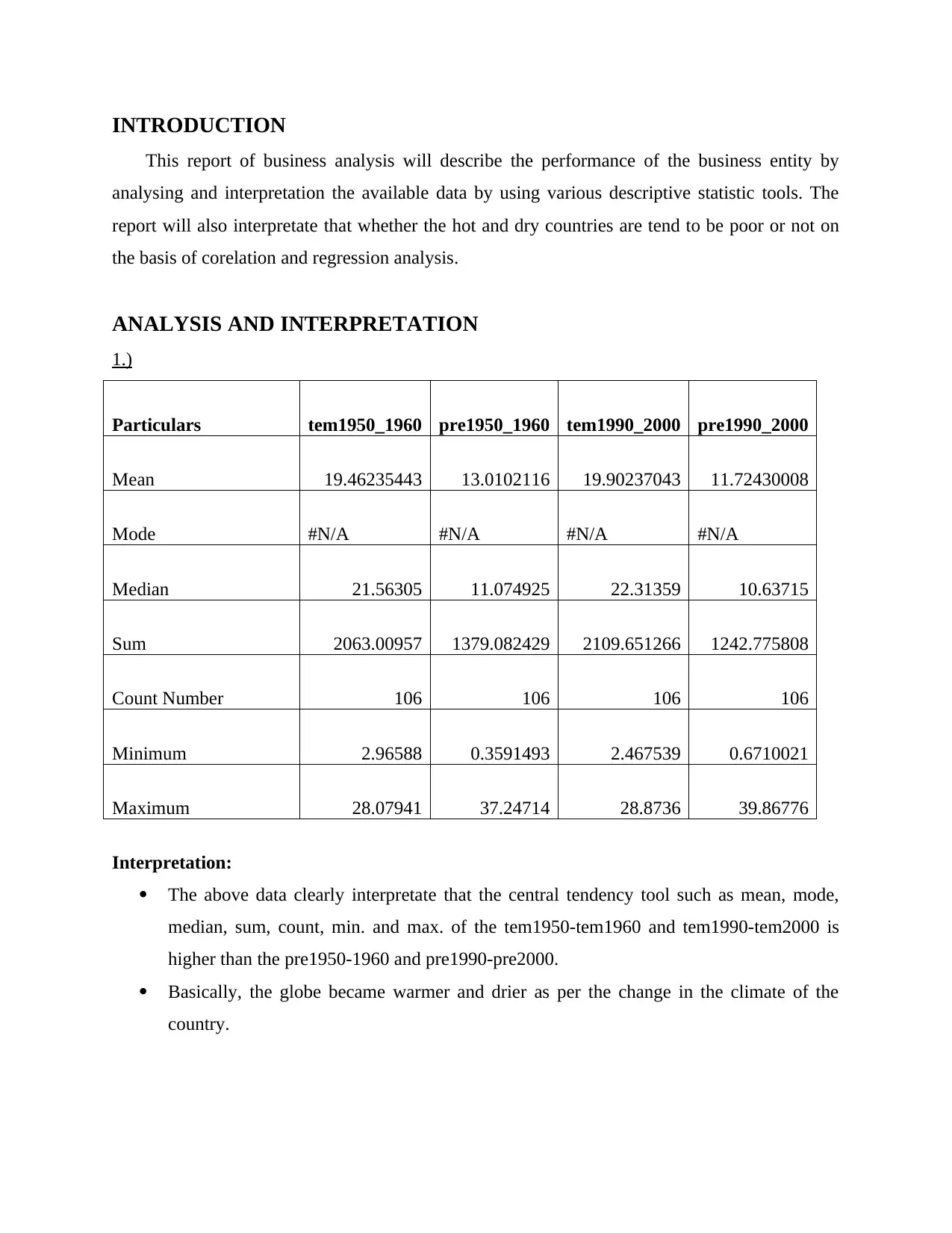
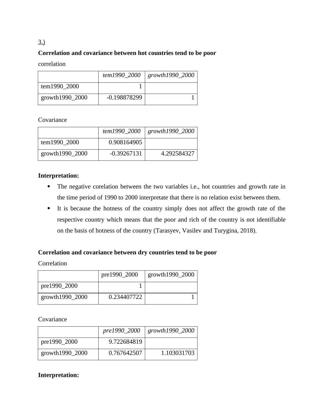
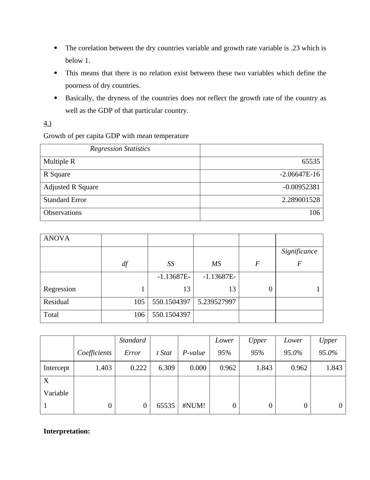
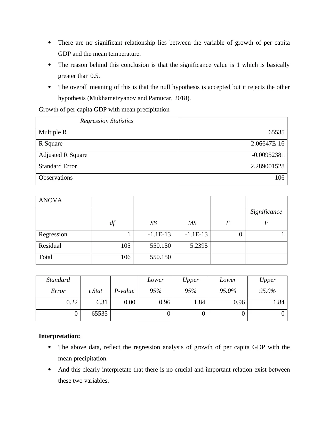
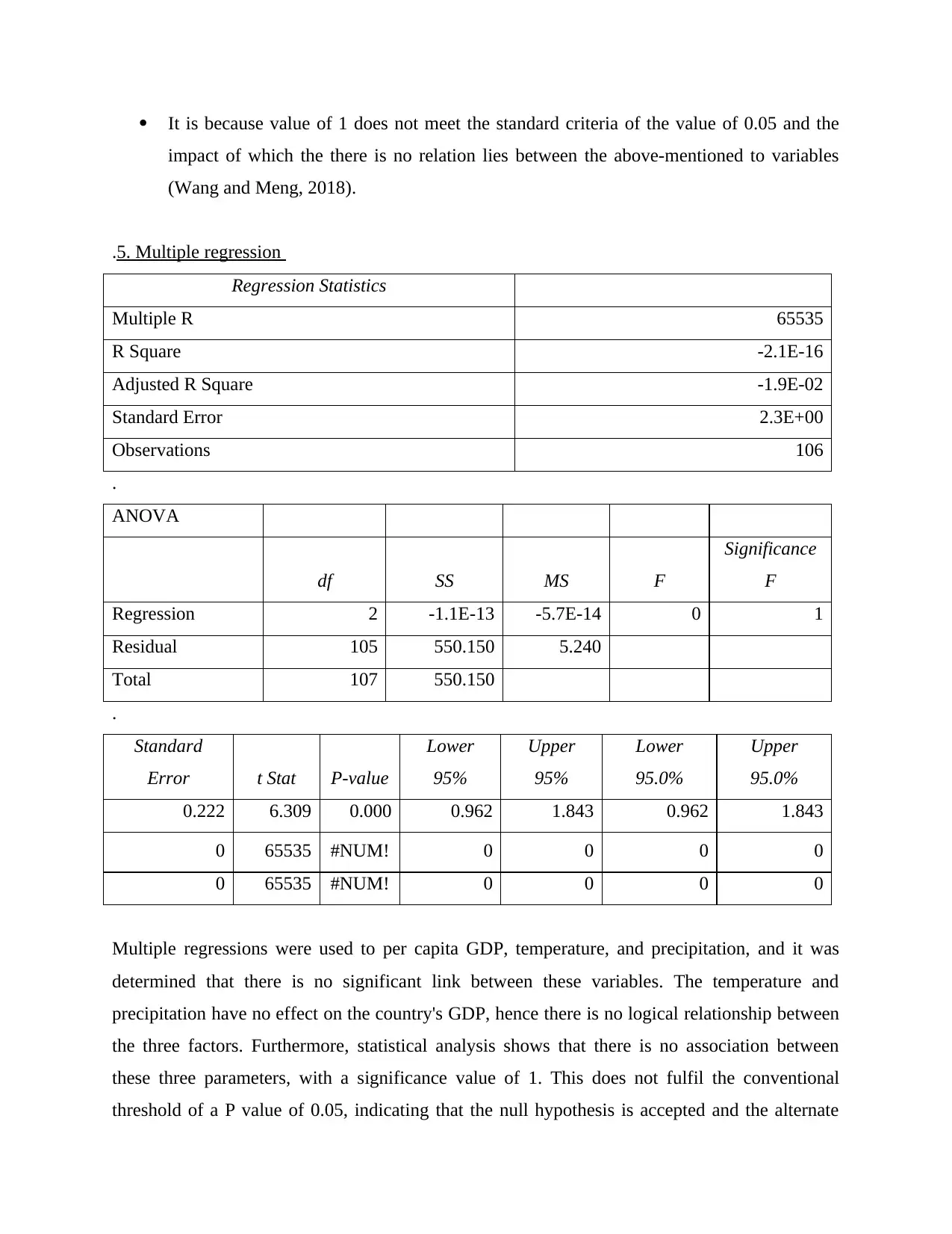
This report presents a statistical analysis of economic data, focusing on the relationship between GDP, temperature, and precipitation across 106 countries. The analysis employs various statistical tools, including descriptive statistics, correlation, regression, and multiple regression analysis. The study investigates the impact of temperature and precipitation on GDP growth, per capita GDP, and identifies key variables influencing economic performance. The report includes an examination of central tendency measures, correlation and covariance, and hypothesis testing. Findings suggest limited correlation between temperature and growth, and an analysis of variables impacting per capita GDP, such as unemployment and poverty. The report concludes with a summary of the findings and references to supporting literature and data sources, including the use of Microsoft Excel for the statistical analysis. The report aims to provide insights into economic growth patterns and the influence of environmental factors.

STATISTICS

EXECUTIVE SUMMARY
This report has been analysed and interpretated the given data and also defined the
performance of the countries on the basis of their growth rate. The report further has been
analysed the various factors and variable with the GDP and growth rate variable via using
various statistic tools, regression and progression analysis including co-relation and co-variance.

Table of Contents
EXECUTIVE SUMMARY.............................................................................................................2
INTRODUCTION...........................................................................................................................4
ANALYSIS AND INTERPRETATION.........................................................................................4
1.).................................................................................................................................................4
2.).................................................................................................................................................5
3.).................................................................................................................................................9
4.)...............................................................................................................................................10
5. Multiple regression..............................................................................................................12
6. Illustrating the below points...............................................................................................13
7. Analysis of R-squared in the multiple regression.............................................................13
8. Two variables that influence the annual growth of per capita GDP..............................14
CONCLUSION..............................................................................................................................14
REFERENCES................................................................................................................................1

INTRODUCTION
This report of business analysis will describe the performance of the business entity by
analysing and interpretation the available data by using various descriptive statistic tools. The
report will also interpretate that whether the hot and dry countries are tend to be poor or not on
the basis of corelation and regression analysis.
ANALYSIS AND INTERPRETATION
1.)
Particulars tem1950_1960 pre1950_1960 tem1990_2000 pre1990_2000
Mean 19.46235443 13.0102116 19.90237043 11.72430008
Mode #N/A #N/A #N/A #N/A
Median 21.56305 11.074925 22.31359 10.63715
Sum 2063.00957 1379.082429 2109.651266 1242.775808
Count Number 106 106 106 106
Minimum 2.96588 0.3591493 2.467539 0.6710021
Maximum 28.07941 37.24714 28.8736 39.86776
Interpretation:
 The above data clearly interpretate that the central tendency tool such as mean, mode,
median, sum, count, min. and max. of the tem1950-tem1960 and tem1990-tem2000 is
higher than the pre1950-1960 and pre1990-pre2000.
 Basically, the globe became warmer and drier as per the change in the climate of the
country.

 No company are able to remain continuous warner all over the time and remain drier all
over the time. It changes over the period of time but as the central tendency of warmer
globe is high.
 So, this analysis means that the globe is warmer rather than the drier in the given period
of 1950 to 2000 (de Maya, Ahn and Kurt, 2019).
2.)
Hot countries relation with its growth rate
Hot Country tem1990_2000 growth1990_2000
Nigeria 26.85172 0.017646708
Panama 25.11478 3.343584973
United Arab Emirates 26.91433 0.351553339
Sierra Leone 26.19973 2.487687259
Brunei 27.06742 2.300388065
Ghana 26.67841 0.582056958
Cote d'Ivoire 26.26308 1.483790792
India 25.26296 8.655843283
Suriname 26.69649 1.356308293
Senegal 27.44442 -0.034229888

Togo 26.32782 -0.437058263
Philippines 25.64058 1.899129864
Mali 28.47546 1.460227831
Oman 25.76736 2.050550258
Mauritania 28.8736 2.508794623
Trinidad and Tobago 26.05961 0.486085514
Indonesia 25.76939 1.171336005
Belize 25.85874 0.422032291
Cuba 25.33854 2.135885605
Dominican Republic 25.66094 -2.469349752
Nicaragua 26.53195 -0.428450843

Interpretation:
 The above graph and data interpretate that the growth rate of the hot counties is not high
and also the number of hot countries having the high growth rate is low that the number
of hot countries having poor growth rate.
 This indicate that the above-mentioned hot countries are tend to be poor (Mustaqeem and
et.al., 2017).
Dry countries relation with its growth rate
Dry Country pre1990_2000 growth1990_2000
United Arab Emirates 1.263214 0.351553339
Spain 6.297207 2.487687259
Austria 9.221741 2.300388065
Canada 9.385453 0.582056958
Australia 7.964385 2.135885605

Egypt 0.6710021 2.512322923
Turkey 6.115713 2.602163169
Saudi Arabia 0.8200489 1.22463352
Luxembourg 7.092182 3.626749501
Tunisia 4.316459 3.286240995
Mozambique 9.191278 2.790436047
Poland 6.146651 3.769896707
Assumption: It is assumed that the average category of hot countries is above 25 temperature
and average category of dry country is below 10 temperatures.
Interpretation:
 The above data and graph clearly interpretate that the dry countries are tend to be poor at
the time period of 1950 to 2000.
 It is because the number of dry countries having poor growth rate is high than the dry
countries having high growth rate (Westerholt, Gröbe and Burghardt, 2018).

3.)
Correlation and covariance between hot countries tend to be poor
correlation
tem1990_2000 growth1990_2000
tem1990_2000 1
growth1990_2000 -0.198878299 1
Covariance
tem1990_2000 growth1990_2000
tem1990_2000 0.908164905
growth1990_2000 -0.39267131 4.292584327
Interpretation:
 The negative corelation between the two variables i.e., hot countries and growth rate in
the time period of 1990 to 2000 interpretate that there is no relation exist between them.
 It is because the hotness of the country simply does not affect the growth rate of the
respective country which means that the poor and rich of the country is not identifiable
on the basis of hotness of the country (Tarasyev, Vasilev and Turygina, 2018).
Correlation and covariance between dry countries tend to be poor
Correlation
pre1990_2000 growth1990_2000
pre1990_2000 1
growth1990_2000 0.234407722 1
Covariance
pre1990_2000 growth1990_2000
pre1990_2000 9.722684819
growth1990_2000 0.767642507 1.103031703
Interpretation:

 The corelation between the dry countries variable and growth rate variable is .23 which is
below 1.
 This means that there is no relation exist between these two variables which define the
poorness of dry countries.
 Basically, the dryness of the countries does not reflect the growth rate of the country as
well as the GDP of that particular country.
4.)
Growth of per capita GDP with mean temperature
Regression Statistics
Multiple R 65535
R Square -2.06647E-16
Adjusted R Square -0.00952381
Standard Error 2.289001528
Observations 106
ANOVA
df SS MS F
Significance
F
Regression 1
-1.13687E-
13
-1.13687E-
13 0 1
Residual 105 550.1504397 5.239527997
Total 106 550.1504397
Coefficients
Standard
Error t Stat P-value
Lower
95%
Upper
95%
Lower
95.0%
Upper
95.0%
Intercept 1.403 0.222 6.309 0.000 0.962 1.843 0.962 1.843
X
Variable
1 0 0 65535 #NUM! 0 0 0 0
Interpretation:

 There are no significant relationship lies between the variable of growth of per capita
GDP and the mean temperature.
 The reason behind this conclusion is that the significance value is 1 which is basically
greater than 0.5.
 The overall meaning of this is that the null hypothesis is accepted but it rejects the other
hypothesis (Mukhametzyanov and Pamucar, 2018).
Growth of per capita GDP with mean precipitation
Regression Statistics
Multiple R 65535
R Square -2.06647E-16
Adjusted R Square -0.00952381
Standard Error 2.289001528
Observations 106
ANOVA
df SS MS F
Significance
F
Regression 1 -1.1E-13 -1.1E-13 0 1
Residual 105 550.150 5.2395
Total 106 550.150
Standard
Error t Stat P-value
Lower
95%
Upper
95%
Lower
95.0%
Upper
95.0%
0.22 6.31 0.00 0.96 1.84 0.96 1.84
0 65535 0 0 0 0
Interpretation:
 The above data, reflect the regression analysis of growth of per capita GDP with the
mean precipitation.
 And this clearly interpretate that there is no crucial and important relation exist between
these two variables.

 It is because value of 1 does not meet the standard criteria of the value of 0.05 and the
impact of which the there is no relation lies between the above-mentioned to variables
(Wang and Meng, 2018).
.5. Multiple regression
Regression Statistics
Multiple R 65535
R Square -2.1E-16
Adjusted R Square -1.9E-02
Standard Error 2.3E+00
Observations 106
.
ANOVA
df SS MS F
Significance
F
Regression 2 -1.1E-13 -5.7E-14 0 1
Residual 105 550.150 5.240
Total 107 550.150
.
Standard
Error t Stat P-value
Lower
95%
Upper
95%
Lower
95.0%
Upper
95.0%
0.222 6.309 0.000 0.962 1.843 0.962 1.843
0 65535 #NUM! 0 0 0 0
0 65535 #NUM! 0 0 0 0
Multiple regressions were used to per capita GDP, temperature, and precipitation, and it was
determined that there is no significant link between these variables. The temperature and
precipitation have no effect on the country's GDP, hence there is no logical relationship between
the three factors. Furthermore, statistical analysis shows that there is no association between
these three parameters, with a significance value of 1. This does not fulfil the conventional
threshold of a P value of 0.05, indicating that the null hypothesis is accepted and the alternate