Statistics for Business and Finance: GE and IBM Price Index Report

This report presents a statistical analysis of GE and IBM price indexes, examining market trends, volatility, and risk. The analysis includes the calculation of returns, summary statistics, and tests of normality using the Jarque-Bera test. The report compares the risk associated with GE and IBM price indexes using F-tests and compares average returns using z-tests and t-tests. It further calculates excess returns, excess market returns, and applies the Capital Asset Pricing Model (CAPM) using linear regression to assess the sensitivity of returns. The report interprets coefficients, R-squared values, and constructs confidence intervals for slope coefficients. Finally, the report evaluates the neutrality of price returns and analyzes the distribution of error terms using normal probability plots.

Running head: STATISTICS FOR BUSINESS AND FINANCE
Statistics for Business and Finance
Name of the Student:
Name of the University:
Author’s note:

1STATISTICS FOR BUSINESS AND FINANCE
Table of Contents
Introduction:................................................................................................................................................................................................2
Discussion:...................................................................................................................................................................................................2
1. Line Chart of Price indexes:.............................................................................................................................................................2
2. Calculation of return prices of each prices:......................................................................................................................................3
2.a. Calculation of returns of S&P500, GE and IBM:.........................................................................................................................3
2.b. Summary Statistics:......................................................................................................................................................................3
2.c. Test of normality by Jarque – Bera test:.......................................................................................................................................3
3. Testing of average return price of GE:.............................................................................................................................................4
4. Comparison of risk associated to both BA and IBM price indexes:.................................................................................................4
5. Comparing the average returns of GE and IBM investing price indexes:........................................................................................4
6. Calculation of Excess Return and Excess Market Return:...............................................................................................................5
7. CAPM calculation by linear regression method:..............................................................................................................................5
7.a. Estimation of CAPM using linear regression:..............................................................................................................................5
7.b. Interpretation of Coefficients:.......................................................................................................................................................5
7.c. Interpretation of R2:.......................................................................................................................................................................6
7.d. Construction of 95% confidence interval for Slope Efficient:.....................................................................................................6
8. Preferable neutral price return:.........................................................................................................................................................6
9. Normal Probability Plot by Orthogonal Least Square Method:.......................................................................................................6

2STATISTICS FOR BUSINESS AND FINANCE
Introduction:
The report discusses about the volatility and risk market, return and market return that is observed as previous studies. The
report also focuses to refer the method of evaluating the company’s price indexes through its market price movements. The price
indexes for GE and International Business Machines (IBM) has been selected for representing. However, the historical price data of
the individual values from 1st February 2010 and 31st July 2015 cannot illustrate the proper results. Hence, the historical index prices
of S&P500 index and the 10 years’ US Treasury Bill are included in the valuation process for computing the beneficial results.
S&P500 index shows the market summarisation and the 10 years’ US Treasury Bill indicates the risk-free return of the market values.
Discussion:
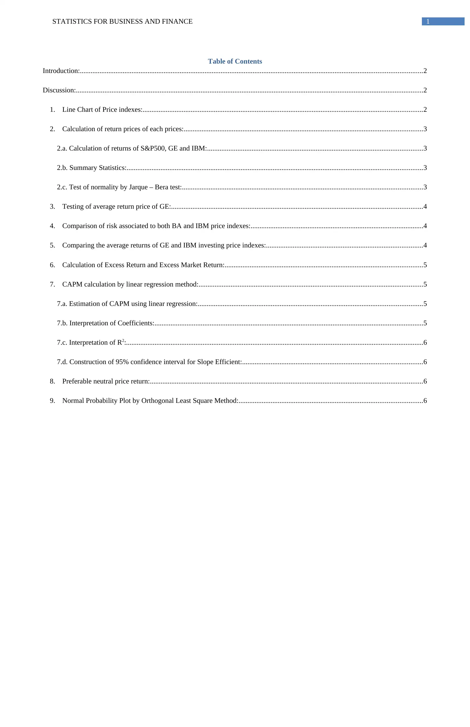
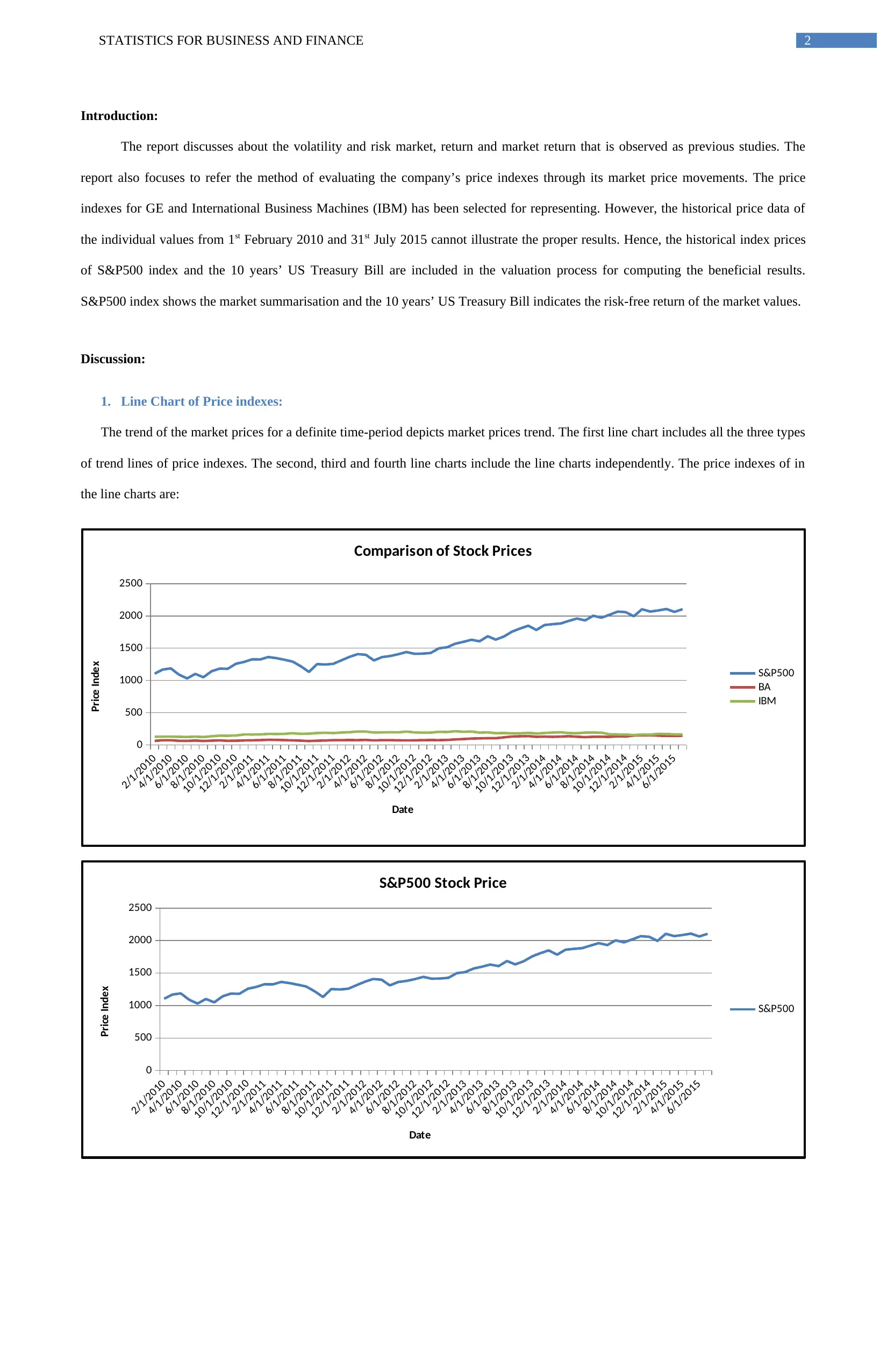
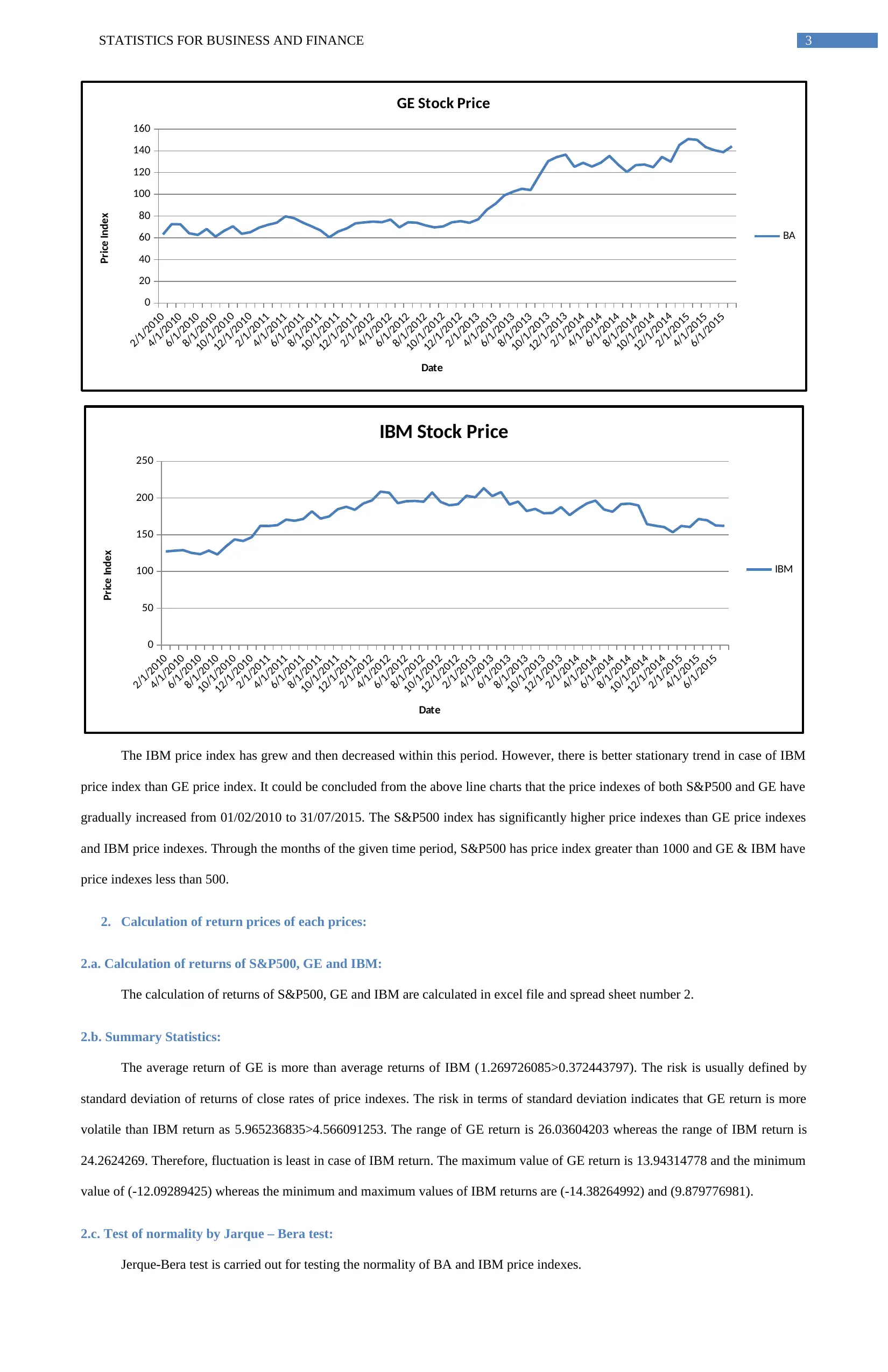
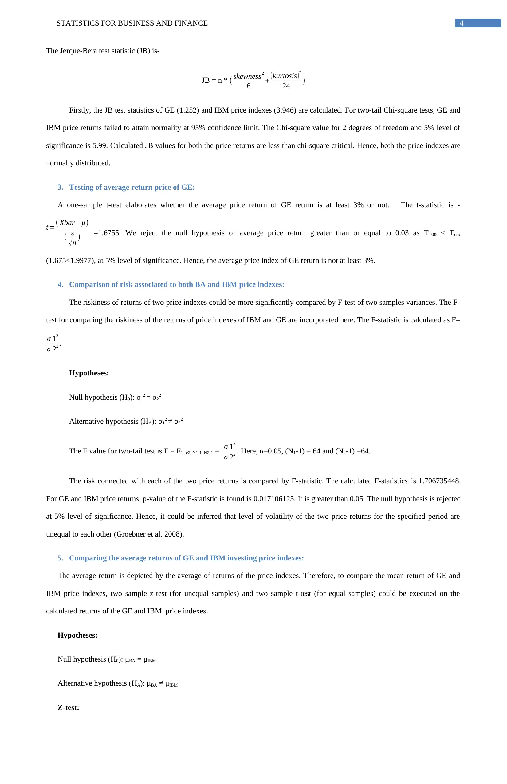
1. Line Chart of Price indexes:
The trend of the market prices for a definite time-period depicts market prices trend. The first line chart includes all the three types
of trend lines of price indexes. The second, third and fourth line charts include the line charts independently. The price indexes of in
the line charts are:
2/1/2010
4/1/2010
6/1/2010
8/1/2010
10/1/2010
12/1/2010
2/1/2011
4/1/2011
6/1/2011
8/1/2011
10/1/2011
12/1/2011
2/1/2012
4/1/2012
6/1/2012
8/1/2012
10/1/2012
12/1/2012
2/1/2013
4/1/2013
6/1/2013
8/1/2013
10/1/2013
12/1/2013
2/1/2014
4/1/2014
6/1/2014
8/1/2014
10/1/2014
12/1/2014
2/1/2015
4/1/2015
6/1/2015
0
500
1000
1500
2000
2500
Comparison of Stock Prices
S&P500
BA
IBM
Date
Price Index
2/1/2010
4/1/2010
6/1/2010
8/1/2010
10/1/2010
12/1/2010
2/1/2011
4/1/2011
6/1/2011
8/1/2011
10/1/2011
12/1/2011
2/1/2012
4/1/2012
6/1/2012
8/1/2012
10/1/2012
12/1/2012
2/1/2013
4/1/2013
6/1/2013
8/1/2013
10/1/2013
12/1/2013
2/1/2014
4/1/2014
6/1/2014
8/1/2014
10/1/2014
12/1/2014
2/1/2015
4/1/2015
6/1/2015
0
500
1000
1500
2000
2500
S&P500 Stock Price
S&P500
Date
Price Index

3STATISTICS FOR BUSINESS AND FINANCE
2/1/2010
4/1/2010
6/1/2010
8/1/2010
10/1/2010
12/1/2010
2/1/2011
4/1/2011
6/1/2011
8/1/2011
10/1/2011
12/1/2011
2/1/2012
4/1/2012
6/1/2012
8/1/2012
10/1/2012
12/1/2012
2/1/2013
4/1/2013
6/1/2013
8/1/2013
10/1/2013
12/1/2013
2/1/2014
4/1/2014
6/1/2014
8/1/2014
10/1/2014
12/1/2014
2/1/2015
4/1/2015
6/1/2015
0
20
40
60
80
100
120
140
160
GE Stock Price
BA
Date
Price Index
2/1/2010
4/1/2010
6/1/2010
8/1/2010
10/1/2010
12/1/2010
2/1/2011
4/1/2011
6/1/2011
8/1/2011
10/1/2011
12/1/2011
2/1/2012
4/1/2012
6/1/2012
8/1/2012
10/1/2012
12/1/2012
2/1/2013
4/1/2013
6/1/2013
8/1/2013
10/1/2013
12/1/2013
2/1/2014
4/1/2014
6/1/2014
8/1/2014
10/1/2014
12/1/2014
2/1/2015
4/1/2015
6/1/2015
0
50
100
150
200
250
IBM Stock Price
IBM
Date
Price Index
The IBM price index has grew and then decreased within this period. However, there is better stationary trend in case of IBM
price index than GE price index. It could be concluded from the above line charts that the price indexes of both S&P500 and GE have
gradually increased from 01/02/2010 to 31/07/2015. The S&P500 index has significantly higher price indexes than GE price indexes
and IBM price indexes. Through the months of the given time period, S&P500 has price index greater than 1000 and GE & IBM have
price indexes less than 500.
2. Calculation of return prices of each prices:
2.a. Calculation of returns of S&P500, GE and IBM:
The calculation of returns of S&P500, GE and IBM are calculated in excel file and spread sheet number 2.
2.b. Summary Statistics:
The average return of GE is more than average returns of IBM (1.269726085>0.372443797). The risk is usually defined by
standard deviation of returns of close rates of price indexes. The risk in terms of standard deviation indicates that GE return is more
volatile than IBM return as 5.965236835>4.566091253. The range of GE return is 26.03604203 whereas the range of IBM return is
24.2624269. Therefore, fluctuation is least in case of IBM return. The maximum value of GE return is 13.94314778 and the minimum
value of (-12.09289425) whereas the minimum and maximum values of IBM returns are (-14.38264992) and (9.879776981).
2.c. Test of normality by Jarque – Bera test:
Jerque-Bera test is carried out for testing the normality of BA and IBM price indexes.

4STATISTICS FOR BUSINESS AND FINANCE
The Jerque-Bera test statistic (JB) is-
JB = n * ( skewness2
6 + ( kurtosis )2
24 )
Firstly, the JB test statistics of GE (1.252) and IBM price indexes (3.946) are calculated. For two-tail Chi-square tests, GE and
IBM price returns failed to attain normality at 95% confidence limit. The Chi-square value for 2 degrees of freedom and 5% level of
significance is 5.99. Calculated JB values for both the price returns are less than chi-square critical. Hence, both the price indexes are
normally distributed.
3. Testing of average return price of GE:
A one-sample t-test elaborates whether the average price return of GE return is at least 3% or not. The t-statistic is -
t=( Xbar−μ)
( s
√ n ) =1.6755. We reject the null hypothesis of average price return greater than or equal to 0.03 as T 0.05 < Tcric
(1.675<1.9977), at 5% level of significance. Hence, the average price index of GE return is not at least 3%.
4. Comparison of risk associated to both BA and IBM price indexes:
The riskiness of returns of two price indexes could be more significantly compared by F-test of two samples variances. The F-
test for comparing the riskiness of the returns of price indexes of IBM and GE are incorporated here. The F-statistic is calculated as F=
σ 12
σ 22 .
Hypotheses:
Null hypothesis (H0): σ12 = σ22
Alternative hypothesis (HA): σ12 ≠ σ22
The F value for two-tail test is F = F1-α/2, N1-1, N2-1 = σ 12
σ 22 . Here, α=0.05, (N1-1) = 64 and (N2-1) =64.
The risk connected with each of the two price returns is compared by F-statistic. The calculated F-statistics is 1.706735448.
For GE and IBM price returns, p-value of the F-statistic is found is 0.017106125. It is greater than 0.05. The null hypothesis is rejected
at 5% level of significance. Hence, it could be inferred that level of volatility of the two price returns for the specified period are
unequal to each other (Groebner et al. 2008).
5. Comparing the average returns of GE and IBM investing price indexes:
The average return is depicted by the average of returns of the price indexes. Therefore, to compare the mean return of GE and
IBM price indexes, two sample z-test (for unequal samples) and two sample t-test (for equal samples) could be executed on the
calculated returns of the GE and IBM price indexes.
Hypotheses:
Null hypothesis (H0): μBA = μIBM
Alternative hypothesis (HA): μBA ≠ μIBM
Z-test:

5STATISTICS FOR BUSINESS AND FINANCE
The z-statistic is given as z¿ ( Xbar −μ)
( σ
√n ) .
For comparing the average returns of each of the two investing price indexes, a z-test is applied. The variances are known for
each of the price returns (GE=35.5840505 and IBM=20.84918933). The calculated z-statistic is 0.962982249. The p-value for two-tail
z-statistic is 0.335556432 (>0.05). Therefore, we can reject the null hypothesis of equality of averages of returns of two price indexes
at 5% level of significance.
Two sample t-test for unequal variances:
The two-sample t-statistic is given by the statistic, t=
( xbar− ybar ) −( μx−μy )
√( sx2
nx ¿ +sy2
ny )¿ .
The t-test assuming equal variances of GE and IBM price returns provide the t-statistic 0.962982249. The p-value of the two-
tail t-test is 0.337492954. The level of significance is 5%, which is lesser than calculated p-value. Therefore, we accept the null
hypothesis of equality of averages of both the price returns.
Decision-making:
In accordance to the price return averages and price return standard deviations (risk), equality is established. Hence, we cannot
draw firm conclusion to select any one price indexes between GE and IBM. Therefore, we proceed with both of them. Subsequently,
we are willing to price excess return, excess market return and CAPM of both the price returns. With the help of these, we can
discover the volatility of both the price returns. The preferable price index would be identified after that.
6. Calculation of Excess Return and Excess Market Return:
The excess return and excess market returns are calculated in the spreadsheet 4 of excel file.
7. CAPM calculation by linear regression method:
The Capital Asset Pricing Model (CAPM) is known as CAPM that is one of the fundamental models in the financial field. The
CAPM illustrates variability in the rate of return (rt) as a function of the rate of return on a market portfolio (rM,t) involving all publicly
traded price indexes. Particularly, the bête (slope) measures the sensitivity of variation of given return of security in the whole market.
Value of beta defines whether the price return is a defensive, a neutral price index or an aggressive price index. Including an intercept
(β0) and an error term (ut) in the model, we have a simple linear regression model –
(rt - rf,t) = β0 + βM (rM,t - rf,t) +ut ………………..(1)
7.a. Estimation of CAPM using linear regression:
The regression models are –
GE excess return = 0.380 + (1.072)*Excess Market Return
IBM excess return = (-1.17) + 0.61*Excess Market Return
7.b. Interpretation of Coefficients:
The calculated beta-value for GE excess return and Excess market return is 1.07210473. The calculated beta-value for IBM excess
return and Excess market return is 0.60966663. The calculated beta-values define that GE price returns have volatility level of

6STATISTICS FOR BUSINESS AND FINANCE
107.21% of the market, whereas the volatility level of IBM compared to the market is 60.96%. Therefore, it can be stated that GE is
highly volatile than IBM. Hence, GE return is considered more profitable than IBM price indexes.
7.c. Interpretation of R2:
The simple linear regression describe that the values of R2 of GE and IBM are 0.43174625 and 0.245170477. The R2 infers the
association of the dependent variable with the independent variable. Therefore, from the values of R2 of the two price returns it can be
concluded that GE excess return (43.17%) is more related than the association of IBM (24.51%).
7.d. Construction of 95% confidence interval for Slope Efficient:
Confidence Interval of IBM Price returns:
A. For GE price returns, slope (β1) = 1.07210473, Standard Error = 0.154961497, d.f. = 64, t-value = 6.918523. Hence, the 95%
confidence interval for the slope coefficient would be (0.762438892, 1.381770571).
B. For IBM price returns, slope (β1) = 0.60966663, Standard Error = 0.134775981, d.f. = 64, t-value = 4.523555. Hence, the 95%
confidence interval for the slope coefficient would be (0.3403383, 0.87899494).
8. Preferable neutral price return:
The testing of aggressiveness of the price returns needs the following hypothesis:
Null hypothesis (H0): β1 = 1
Alternative hypothesis (H1): β1 < 1
For both the price returns, the p-values are positive t-value and equal degrees of freedom 64. The 95% confidence intervals for
beta values of both BA and IBM price returns are (0.762438892, 1.381770571) and (0.3403383, 0.87899494). The confidence
intervals near to 0 indicates more neutral nature for price exchange return. The confidence intervals of t-statistics show that IBM price
return is more neutral.
9. Normal Probability Plot by Orthogonal Least Square Method:
The method of ordinary least squares (OLS) helps to establish the normality with diagrams. The error terms in the model are
graphically indicated in normal probability plot. The distribution of residual values is symmetric for the market return values. It
shows that the error terms are not following normal distributions for IBm price returns.
Besides the Jerque-bera test of the residual values of IBM excess price returns, indicate that JB test statistic is 2.664 for IBM
price indexes due to predicted excess value. For chi-square distribution of 2 degrees of freedom at 5% level of significance, the chi-
square statistic is 5.99. Therefore, we accept the normality of residual values of IBM price indexes.