Statistical Inference, Correlation, and Regression Analysis: Findings

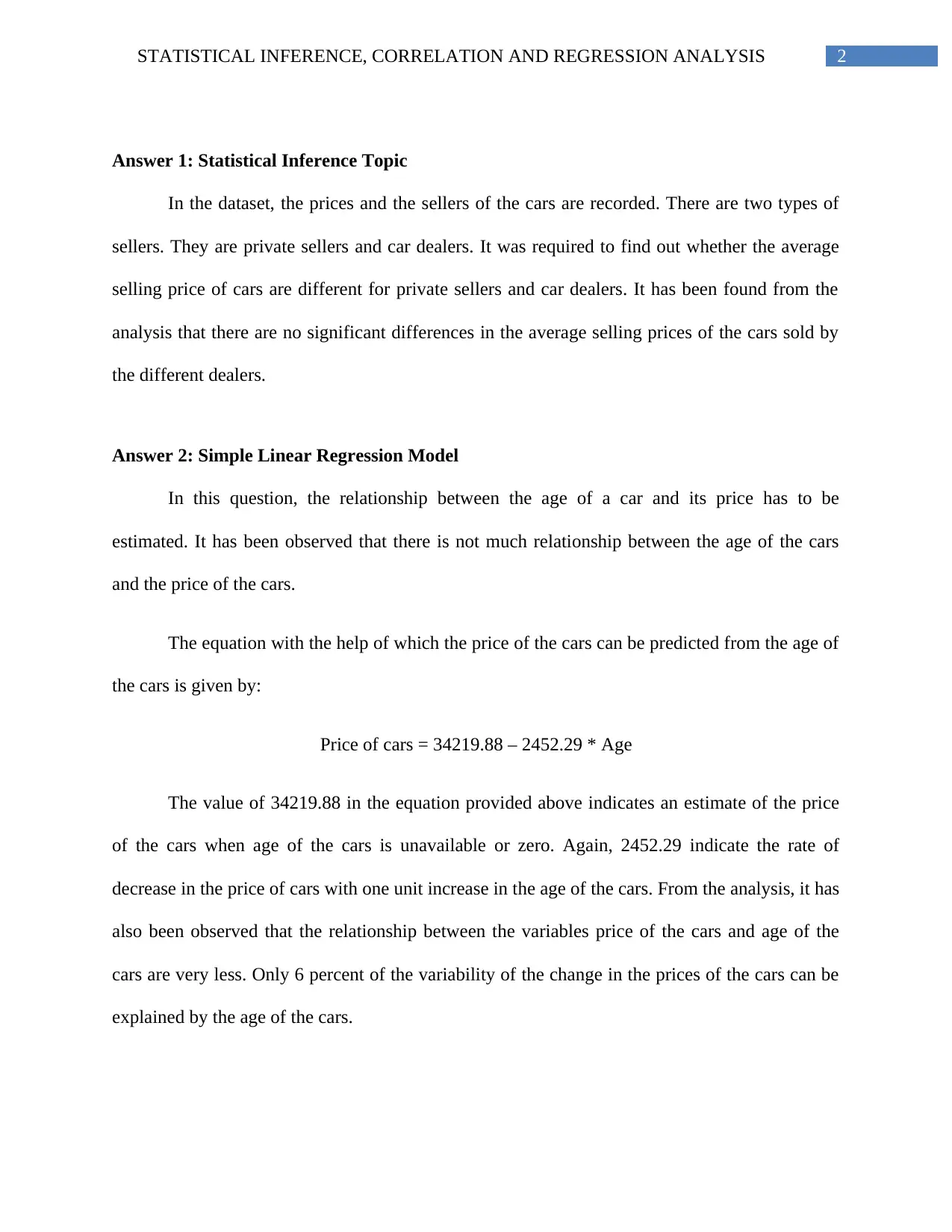
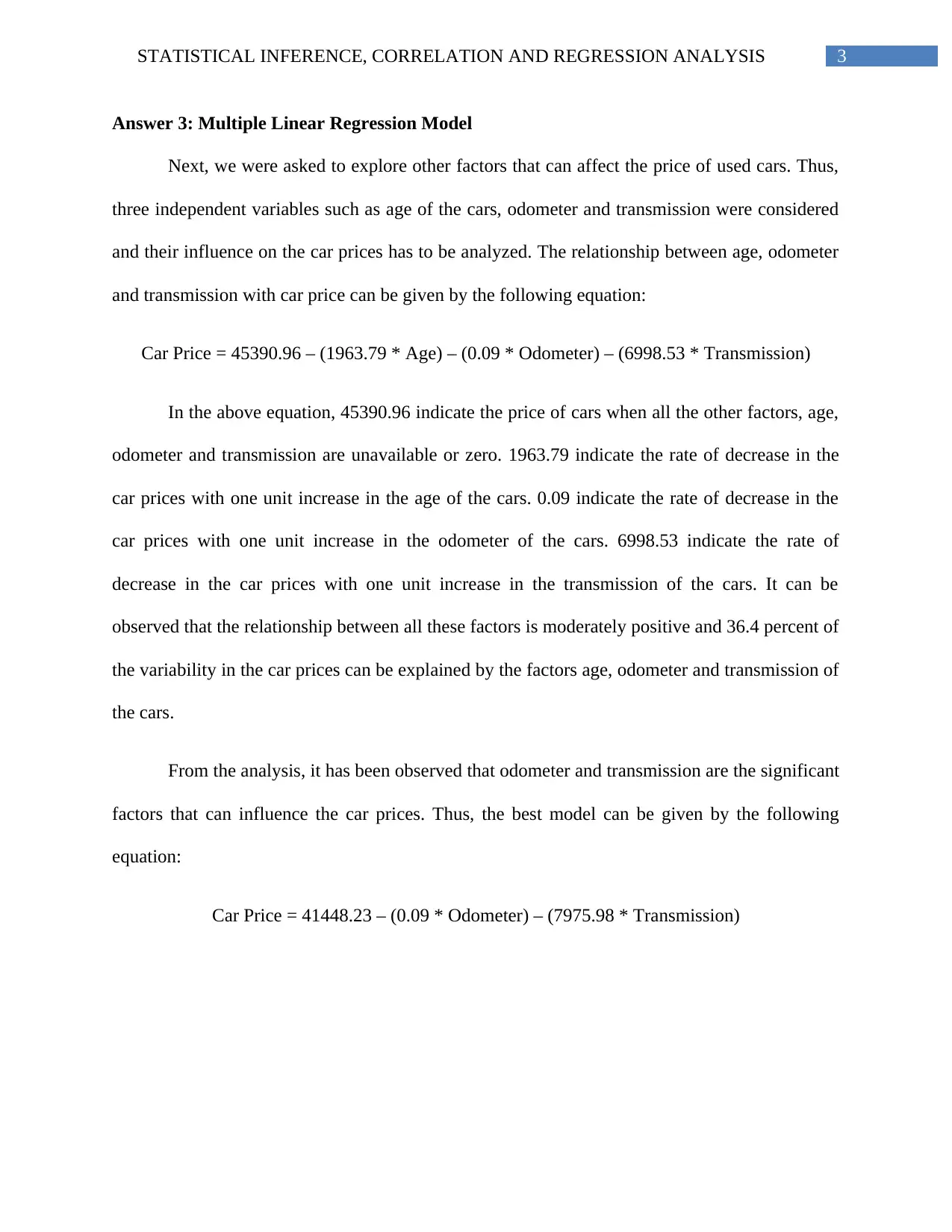
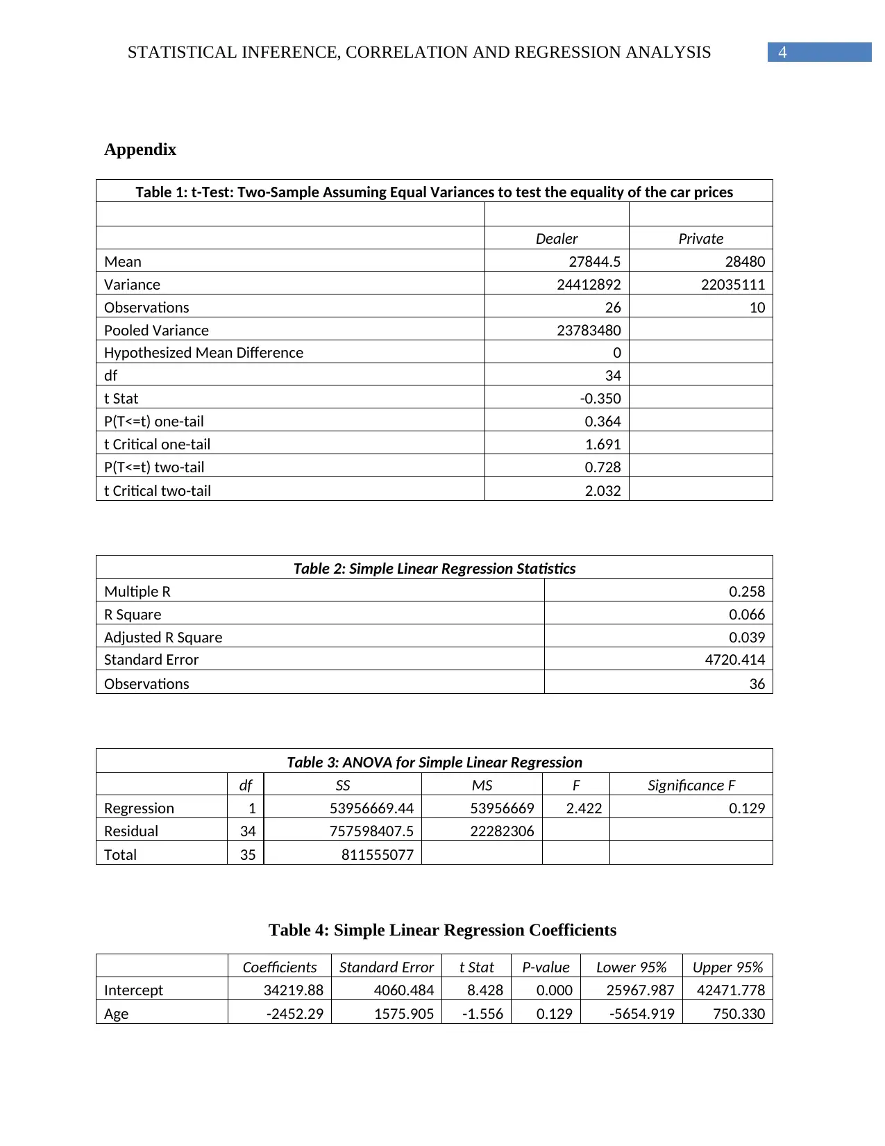
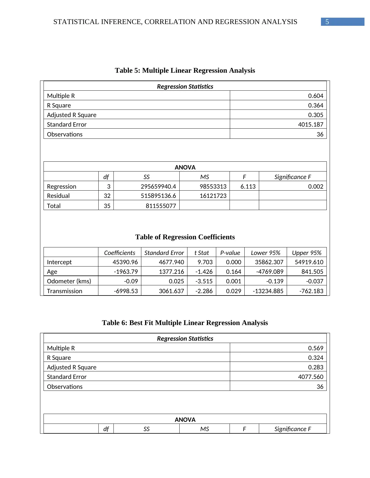
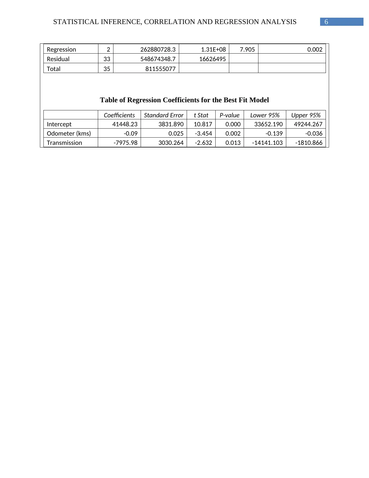
This assignment presents a statistical analysis of car prices, exploring the application of statistical inference, correlation, and regression models. The analysis begins by investigating whether there are significant differences in the average selling prices of cars sold by private sellers versus car dealers, finding no significant differences. Subsequently, a simple linear regression model is employed to estimate the relationship between car age and price, revealing a weak correlation, with only 6% of price variability explained by age. The equation for this model is provided, along with interpretations of the coefficients. A multiple linear regression model is then developed, incorporating age, odometer reading, and transmission type as independent variables. The analysis reveals that odometer and transmission are significant factors influencing car prices, and the best-fit model is presented, along with its corresponding equation. The report includes several tables of regression coefficients and ANOVA results to support the findings.

Running Head: STATISTICAL INFERENCE, CORRELATION AND REGRESSION
ANALYSIS
Statistical Inference, Correlation and Regression Analysis
Name of the Student
Name of the University
Author Note

1STATISTICAL INFERENCE, CORRELATION AND REGRESSION ANALYSIS
Table of Contents
Answer 1: Statistical Inference Topic..............................................................................................2
Answer 2: Simple Linear Regression Model...................................................................................2
Answer 3: Multiple Linear Regression Model................................................................................2

2STATISTICAL INFERENCE, CORRELATION AND REGRESSION ANALYSIS
Answer 1: Statistical Inference Topic
In the dataset, the prices and the sellers of the cars are recorded. There are two types of
sellers. They are private sellers and car dealers. It was required to find out whether the average
selling price of cars are different for private sellers and car dealers. It has been found from the
analysis that there are no significant differences in the average selling prices of the cars sold by
the different dealers.
Answer 2: Simple Linear Regression Model
In this question, the relationship between the age of a car and its price has to be
estimated. It has been observed that there is not much relationship between the age of the cars
and the price of the cars.
The equation with the help of which the price of the cars can be predicted from the age of
the cars is given by:
Price of cars = 34219.88 – 2452.29 * Age
The value of 34219.88 in the equation provided above indicates an estimate of the price
of the cars when age of the cars is unavailable or zero. Again, 2452.29 indicate the rate of
decrease in the price of cars with one unit increase in the age of the cars. From the analysis, it has
also been observed that the relationship between the variables price of the cars and age of the
cars are very less. Only 6 percent of the variability of the change in the prices of the cars can be
explained by the age of the cars.

3STATISTICAL INFERENCE, CORRELATION AND REGRESSION ANALYSIS
Answer 3: Multiple Linear Regression Model
Next, we were asked to explore other factors that can affect the price of used cars. Thus,
three independent variables such as age of the cars, odometer and transmission were considered
and their influence on the car prices has to be analyzed. The relationship between age, odometer
and transmission with car price can be given by the following equation:
Car Price = 45390.96 – (1963.79 * Age) – (0.09 * Odometer) – (6998.53 * Transmission)
In the above equation, 45390.96 indicate the price of cars when all the other factors, age,
odometer and transmission are unavailable or zero. 1963.79 indicate the rate of decrease in the
car prices with one unit increase in the age of the cars. 0.09 indicate the rate of decrease in the
car prices with one unit increase in the odometer of the cars. 6998.53 indicate the rate of
decrease in the car prices with one unit increase in the transmission of the cars. It can be
observed that the relationship between all these factors is moderately positive and 36.4 percent of
the variability in the car prices can be explained by the factors age, odometer and transmission of
the cars.
From the analysis, it has been observed that odometer and transmission are the significant
factors that can influence the car prices. Thus, the best model can be given by the following
equation:
Car Price = 41448.23 – (0.09 * Odometer) – (7975.98 * Transmission)

4STATISTICAL INFERENCE, CORRELATION AND REGRESSION ANALYSIS
Appendix
Table 1: t-Test: Two-Sample Assuming Equal Variances to test the equality of the car prices
Dealer Private
Mean 27844.5 28480
Variance 24412892 22035111
Observations 26 10
Pooled Variance 23783480
Hypothesized Mean Difference 0
df 34
t Stat -0.350
P(T<=t) one-tail 0.364
t Critical one-tail 1.691
P(T<=t) two-tail 0.728
t Critical two-tail 2.032
Table 2: Simple Linear Regression Statistics
Multiple R 0.258
R Square 0.066
Adjusted R Square 0.039
Standard Error 4720.414
Observations 36
Table 3: ANOVA for Simple Linear Regression
df SS MS F Significance F
Regression 1 53956669.44 53956669 2.422 0.129
Residual 34 757598407.5 22282306
Total 35 811555077
Table 4: Simple Linear Regression Coefficients
Coefficients Standard Error t Stat P-value Lower 95% Upper 95%
Intercept 34219.88 4060.484 8.428 0.000 25967.987 42471.778
Age -2452.29 1575.905 -1.556 0.129 -5654.919 750.330

5STATISTICAL INFERENCE, CORRELATION AND REGRESSION ANALYSIS
Table 5: Multiple Linear Regression Analysis
Regression Statistics
Multiple R 0.604
R Square 0.364
Adjusted R Square 0.305
Standard Error 4015.187
Observations 36
ANOVA
df SS MS F Significance F
Regression 3 295659940.4 98553313 6.113 0.002
Residual 32 515895136.6 16121723
Total 35 811555077
Table of Regression Coefficients
Coefficients Standard Error t Stat P-value Lower 95% Upper 95%
Intercept 45390.96 4677.940 9.703 0.000 35862.307 54919.610
Age -1963.79 1377.216 -1.426 0.164 -4769.089 841.505
Odometer (kms) -0.09 0.025 -3.515 0.001 -0.139 -0.037
Transmission -6998.53 3061.637 -2.286 0.029 -13234.885 -762.183
Table 6: Best Fit Multiple Linear Regression Analysis
Regression Statistics
Multiple R 0.569
R Square 0.324
Adjusted R Square 0.283
Standard Error 4077.560
Observations 36
ANOVA
df SS MS F Significance F

6STATISTICAL INFERENCE, CORRELATION AND REGRESSION ANALYSIS
Regression 2 262880728.3 1.31E+08 7.905 0.002
Residual 33 548674348.7 16626495
Total 35 811555077
Table of Regression Coefficients for the Best Fit Model
Coefficients Standard Error t Stat P-value Lower 95% Upper 95%
Intercept 41448.23 3831.890 10.817 0.000 33652.190 49244.267
Odometer (kms) -0.09 0.025 -3.454 0.002 -0.139 -0.036
Transmission -7975.98 3030.264 -2.632 0.013 -14141.103 -1810.866