Analysis of Economic and Business Data: Statistics for Management

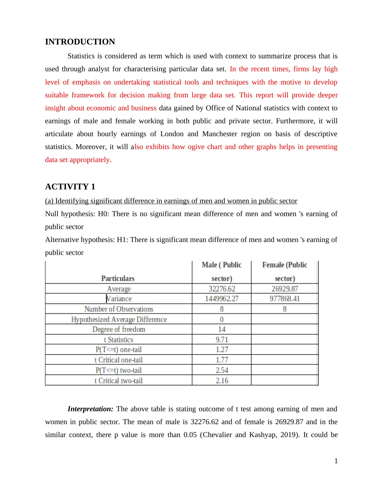
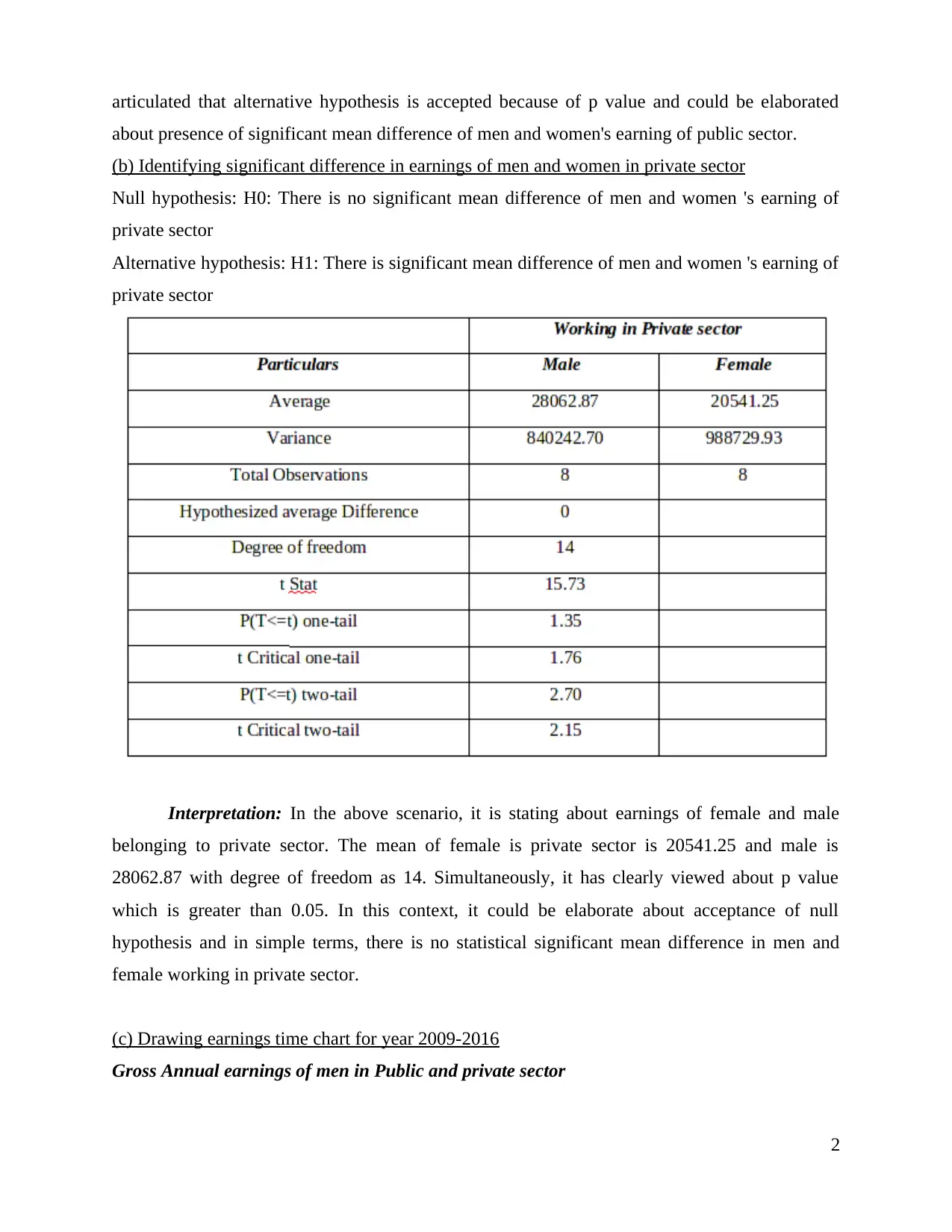
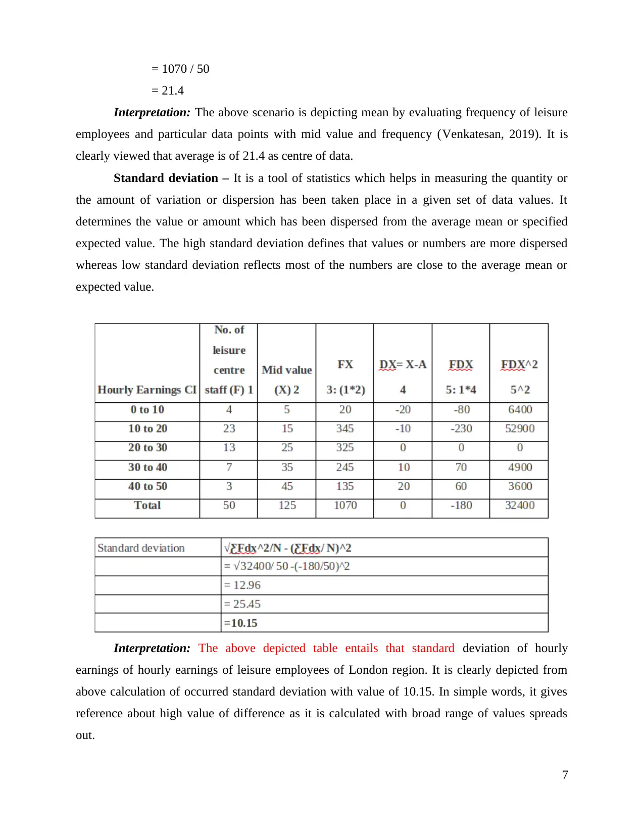
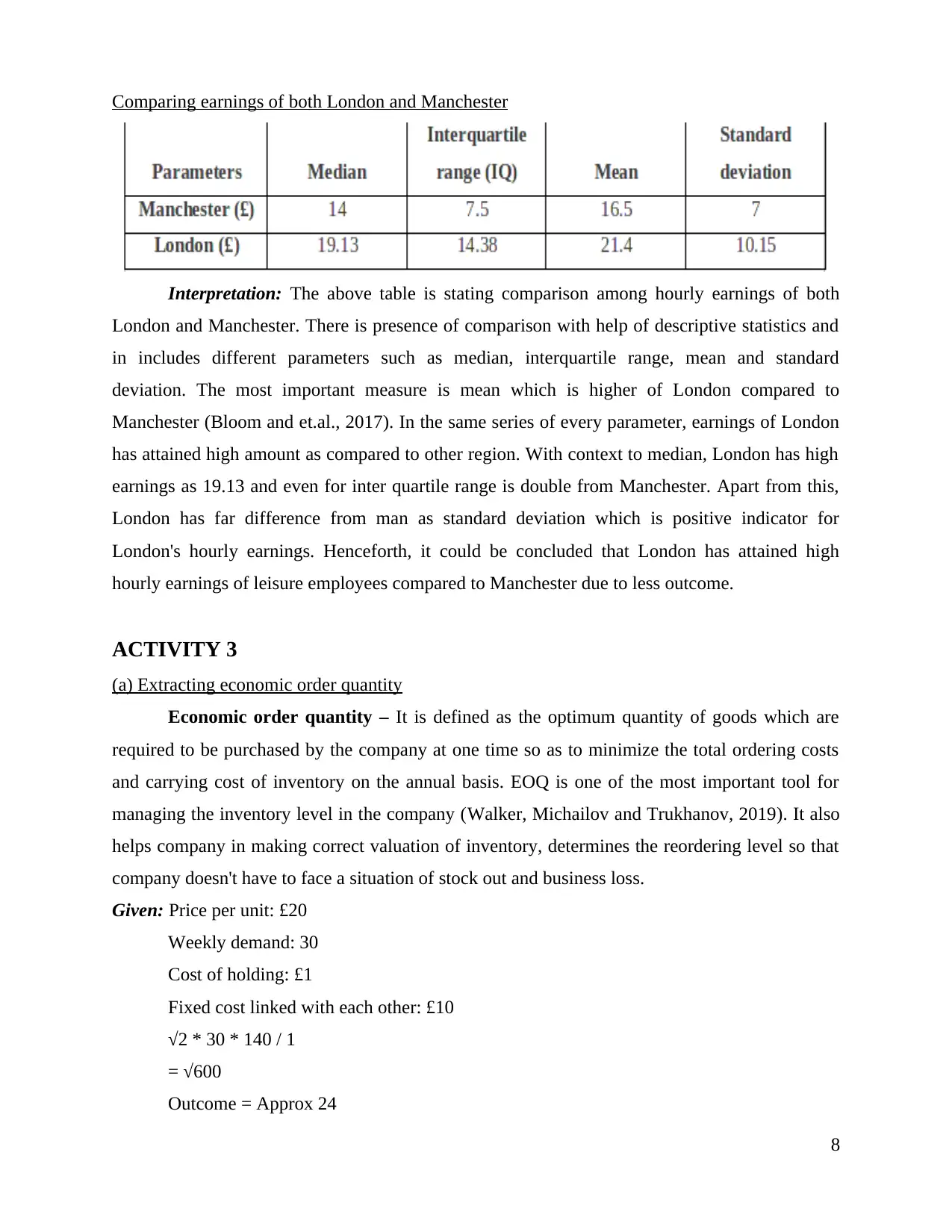
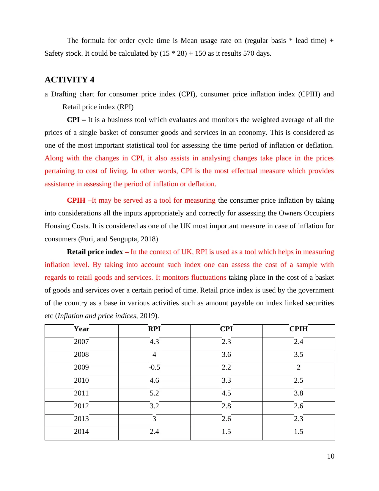
This report provides a comprehensive statistical analysis of economic and business data. It begins by comparing earnings between men and women in both public and private sectors using t-tests, followed by a time chart analysis of gross annual earnings. Descriptive statistics, including ogive charts, are employed to determine median hourly earnings, quartiles, mean, and standard deviation for London and Manchester regions. The report further explores inventory management, calculating economic order quantity (EOQ), order and cost analysis, and service levels. Finally, it presents an analysis of consumer price indices (CPI, CPIH, RPI) and their trends, along with an ogive chart illustrating cumulative staff percentages versus hourly earnings, offering valuable insights into financial and economic indicators. The report uses data from the Office of National Statistics and covers topics such as the identification of significant differences in earnings, the use of ogive charts, the calculation of economic order quantity, and the analysis of consumer price indices.

STATISTICS FOR
MANAGEMENT

INTRODUCTION
Statistics is considered as term which is used with context to summarize process that is
used through analyst for characterising particular data set. In the recent times, firms lay high
level of emphasis on undertaking statistical tools and techniques with the motive to develop
suitable framework for decision making from large data set. This report will provide deeper
insight about economic and business data gained by Office of National statistics with context to
earnings of male and female working in both public and private sector. Furthermore, it will
articulate about hourly earnings of London and Manchester region on basis of descriptive
statistics. Moreover, it will also exhibits how ogive chart and other graphs helps in presenting
data set appropriately.
ACTIVITY 1
(a) Identifying significant difference in earnings of men and women in public sector
Null hypothesis: H0: There is no significant mean difference of men and women 's earning of
public sector
Alternative hypothesis: H1: There is significant mean difference of men and women 's earning of
public sector
Interpretation: The above table is stating outcome of t test among earning of men and
women in public sector. The mean of male is 32276.62 and of female is 26929.87 and in the
similar context, there p value is more than 0.05 (Chevalier and Kashyap, 2019). It could be
1

articulated that alternative hypothesis is accepted because of p value and could be elaborated
about presence of significant mean difference of men and women's earning of public sector.
(b) Identifying significant difference in earnings of men and women in private sector
Null hypothesis: H0: There is no significant mean difference of men and women 's earning of
private sector
Alternative hypothesis: H1: There is significant mean difference of men and women 's earning of
private sector
Interpretation: In the above scenario, it is stating about earnings of female and male
belonging to private sector. The mean of female is private sector is 20541.25 and male is
28062.87 with degree of freedom as 14. Simultaneously, it has clearly viewed about p value
which is greater than 0.05. In this context, it could be elaborate about acceptance of null
hypothesis and in simple terms, there is no statistical significant mean difference in men and
female working in private sector.
(c) Drawing earnings time chart for year 2009-2016
Gross Annual earnings of men in Public and private sector
2

Gross Annual earnings of women in Public and private sector
3

(d) Identifying annual growth rate in earnings of all four groups
ACTIVITY 2
(I) Using ogive, estimate median hourly earnings along with quartiles
Ogive – It is also known as Cumulative histogram which is defined as a cumulative
frequency graph. With the help of this cumulative frequency graph, one can determine the
number of data points which are equal to or are below a certain specified value in the given data
set. The most important use of Ogive is for determining the median and percentiles of the given
set of data (Bzdok, Altman and Krzywinski, 2018). It is a graph which shows the curve of a
cumulative distribution function and the points plotted are upper class limit and corresponding
cumulative frequency.
4

Median of London region
L+ Cf-n/ f* I
= 10+(20-10)/ 23 * (25 - 4)
= 10 + ((10*21)/23)
= 10 + (210/23)
= 10+ 9.13
= 19.13
Interpretation: The above table and graph is reflecting ogive chart with objective to
articulate median for hourly earnings of London region. It has clearly shown cumulative is
raising towards right and on the contrary, number of leisure staff increased till 10 to 20 but
5

afterwards it decreased on gradual basis (Nisar, Prabhakar and Strakova, 2019). Generally, ogive
is one of the easiest and best way to articulate median which results 19.13.
Quartile
Quartile Method Result
Q1 10 + ((20-10)/23)*(12.5 – 4)
= 10 + (10/23) * 8.5
= 10+ 3.70
13.7
Q2 19.13
Q3 20 + ((30-20)/23)*(37.5 – 27)
= 20 + (10/13) * 10.5
= 20 + 8.08
28.08
Interquartile range Q3 – Q1
28.08 – 13.70
14.38
Interpretation: Tabular presentation shows that quartile of hourly earnings of leisure
employees of London region as Quartile 1 is 13.7 which replicates that 25% of data is less than
13.7 and remaining 75% is more than this. Simultaneously, quartile 2 is 19.13 which itself is
median of data set as half data and quartile 3 is 28.08 as 75th percentile whereas 25% data is
higher and remaining is smaller.
(ii) Calculating standard deviation and mean for hourly earnings
Mean
Mean formula: Sum of FX / Total number of data points
6

= 1070 / 50
= 21.4
Interpretation: The above scenario is depicting mean by evaluating frequency of leisure
employees and particular data points with mid value and frequency (Venkatesan, 2019). It is
clearly viewed that average is of 21.4 as centre of data.
Standard deviation – It is a tool of statistics which helps in measuring the quantity or
the amount of variation or dispersion has been taken place in a given set of data values. It
determines the value or amount which has been dispersed from the average mean or specified
expected value. The high standard deviation defines that values or numbers are more dispersed
whereas low standard deviation reflects most of the numbers are close to the average mean or
expected value.
Interpretation: The above depicted table entails that standard deviation of hourly
earnings of hourly earnings of leisure employees of London region. It is clearly depicted from
above calculation of occurred standard deviation with value of 10.15. In simple words, it gives
reference about high value of difference as it is calculated with broad range of values spreads
out.
7

Comparing earnings of both London and Manchester
Interpretation: The above table is stating comparison among hourly earnings of both
London and Manchester. There is presence of comparison with help of descriptive statistics and
in includes different parameters such as median, interquartile range, mean and standard
deviation. The most important measure is mean which is higher of London compared to
Manchester (Bloom and et.al., 2017). In the same series of every parameter, earnings of London
has attained high amount as compared to other region. With context to median, London has high
earnings as 19.13 and even for inter quartile range is double from Manchester. Apart from this,
London has far difference from man as standard deviation which is positive indicator for
London's hourly earnings. Henceforth, it could be concluded that London has attained high
hourly earnings of leisure employees compared to Manchester due to less outcome.
ACTIVITY 3
(a) Extracting economic order quantity
Economic order quantity – It is defined as the optimum quantity of goods which are
required to be purchased by the company at one time so as to minimize the total ordering costs
and carrying cost of inventory on the annual basis. EOQ is one of the most important tool for
managing the inventory level in the company (Walker, Michailov and Trukhanov, 2019). It also
helps company in making correct valuation of inventory, determines the reordering level so that
company doesn't have to face a situation of stock out and business loss.
Given: Price per unit: £20
Weekly demand: 30
Cost of holding: £1
Fixed cost linked with each other: £10
√2 * 30 * 140 / 1
= √600
Outcome = Approx 24
8

(b) Order and cost
In the given scenario, 117 t shirts could be implied till 2.3 weeks as its elaboration is
stated below:
117 / 55
23 weeks
Yearly demand for t shirts: 50* 55
Yearly demand= 2750
As per duration to order t shirts are 2750/ 17
24 times
(c) Inventory policy cost
Size of order is of 117 units as number of orders are calculated as 250/ 117 which results
23.5 orders. Moreover, ordering cost is 23.5 * 5 as 117.5 and mean inventory level is calculated
in units as (3370 + 0)/ 2 gives result 168.5.
In the same series, there is articulation of holding and inventory cost as 168.5 is
multiplied by 2 is 337 and 117.5 + 337 as 454.5 or 455 t shirts respectively.
(d) Current service level
The current level of service is articulated as 150 as:
Z= (37.05 – 30) / 15
= 0.5
=0.5 or 50%= 0.195 or 19.15%50% + 19.15%
= 50% + 19.15%
= 69.15% as current level of service.
On basis of above assessment, it could be articulated that t shirts must be in stock with approx of
69.15% of times. Thus, remaining 30.85% of time business could directly avoid maintenance of
stock of t-shirt.
(e) Extracting re-order level
Re-order level is known as inventory level at which business would place new order or
would directly initiate with manufacturing or production of services and goods. Generally, it is
dependent on lead time of work of company along with demand during particular duration
(Koutras, Koutras. and Yalcin, 2016). It analyses the maintenance of safety stock or not as initial
reason to extract reorder point is to recognise when amount for particular products has dropped
level of point where business has other request through provider.
9

The formula for order cycle time is Mean usage rate on (regular basis * lead time) +
Safety stock. It could be calculated by (15 * 28) + 150 as it results 570 days.
ACTIVITY 4
a Drafting chart for consumer price index (CPI), consumer price inflation index (CPIH) and
Retail price index (RPI)
CPI – It is a business tool which evaluates and monitors the weighted average of all the
prices of a single basket of consumer goods and services in an economy. This is considered as
one of the most important statistical tool for assessing the time period of inflation or deflation.
Along with the changes in CPI, it also assists in analysing changes take place in the prices
pertaining to cost of living. In other words, CPI is the most effectual measure which provides
assistance in assessing the period of inflation or deflation.
CPIH –It may be served as a tool for measuring the consumer price inflation by taking
into considerations all the inputs appropriately and correctly for assessing the Owners Occupiers
Housing Costs. It is considered as one of the UK most important measure in case of inflation for
consumers (Puri, and Sengupta, 2018)
Retail price index – In the context of UK, RPI is used as a tool which helps in measuring
inflation level. By taking into account such index one can assess the cost of a sample with
regards to retail goods and services. It monitors fluctuations taking place in the cost of a basket
of goods and services over a certain period of time. Retail price index is used by the government
of the country as a base in various activities such as amount payable on index linked securities
etc (Inflation and price indices, 2019).
Year RPI CPI CPIH
2007 4.3 2.3 2.4
2008 4 3.6 3.5
2009 -0.5 2.2 2
2010 4.6 3.3 2.5
2011 5.2 4.5 3.8
2012 3.2 2.8 2.6
2013 3 2.6 2.3
2014 2.4 1.5 1.5
10