STAT1060 Assignment 2: Statistical Analysis to Support Decision Making

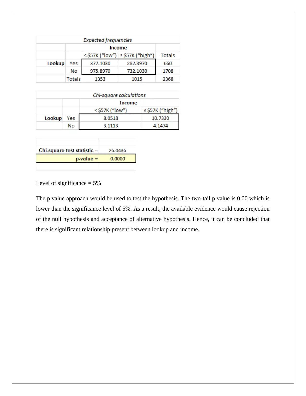
This document presents a comprehensive solution to a statistical analysis assignment (STAT1060, Assignment 2), focusing on applying statistical techniques to real-world data. The solution begins with an analysis of sampling techniques, identifying convenience sampling and its limitations. It then addresses data types, graphical representations like bar charts and histograms, and measures of central tendency and dispersion. The assignment involves analyzing an asset liability ratio dataset, comparing operational and closed businesses, and conducting hypothesis tests to determine significant differences. Furthermore, the solution covers probability calculations, empirical rule application, and the verification of an economist's claim. It also includes hypothesis testing for packaging techniques and the relationship between income and lookup using chi-square tests. The analysis utilizes Excel for computations, generating relevant graphs, and interpreting results to support decision-making. The document provides a clear, step-by-step approach to solving statistical problems, making it an excellent resource for students studying statistics and data analysis.

Question 1
a) The sampling technique used for obtaining the given data would be terms as convenience
sampling which is a non-probability based sampling technique. This is because the responses
have been collected from first 400 responders. No attempt has been made to randomly derive
the sample from population of interest. It is likely that there is bias in the responses thereby
adversely impacting the reliability of the results obtained.
b) The number of cards is a discrete variable since the given variable has a numerical value
which can only assume integer values. This is because number of cards cannot assume
decimal values and hence it is not continuous.
c) The requisite graphical technique to capture the given data is bar chart where for each
number of cards, the corresponding bars would indicate the number of respondents having
these many cards.
d) The requisite graphical summary of the given data is obtained from Excel and illustrated
below.
e) It is evident from the above graphical representation that the distribution of number of cards
seems to have a positive skew. This is because there are a small number of respondents who

have 6 cards which is little unexpected considering that 99% of the respondents have four or
less cards. Also, from the distribution, it is apparent that the most common number of cards
held is 3 which has the largest frequency in the given data.
Question 2
a) Asset liability ratio would be a continuous variable since the underlying values are numerical
and also can assume decimal values and not restricted to only integral values. The
operational variable is nominal since it is a categorical variable which does not assume
numerical value and also the responses are of the type that cannot be arranged in a naturally
occurring order.
b) The requisite histogram for Asset Liability Ratio is shown below.
The above histogram clearly highlights that the shape is not symmetric owing to skew being
present. As a result, the maximum frequency interval does not occur in the middle of the
histogram.

c) A column chart would be used to allow for comparison of Asset Liability Ratio for the closed
and still operational small businesses. This is clearly evident from the following graph
obtained from Excel.
d) The requisite measures of central tendency and dispersion for Asset Liability Ratio have been
computed using Excel and presented below.
e) From the above output, it is evident that there is a significant different between the asset
liability ratio of the operational and closed businesses. The now closed small businesses have
mean and median value of asset liability ratio of about 0.5 which would have been a major
reason for the closure of these businesses. This value implies that the corresponding assets
are significantly lower than the outstanding liabilities thereby indicating inability to meet the

outstanding liabilities. This is not the case with regards to operational small businesses whose
asset liability ratio is quite healthy thereby implying the ability to meet the outstanding
liabilities. There is no significant difference with regards to the variation of asset liability
ratio between the two categories of firms. However, considering the mean, variation in
percentage terms is higher for now closed firms as compared to operational businesses.
f) 1) Mean asset liability ratio for operational firms = 1.73
Standard deviation in the asset liability ratio for operational firms = 0.24
It is evident that the value of 1.97 would corresponding to mean + 1 standard deviation. The
probability of operational firms having more than 1.97 as their asset liability ratio can be
computed using the following graph capturing empirical use.
Hence, requisite probability = 0.135 + 0.0235 = 0.16
2) The validity of the claim of the researcher can be verified by determining the actual
probability using the sample data required and compare the same with the probability
determined using the empirical rule.
Total businesses which are still operational = 53
Number of these businesses where asset liability ratio exceeds 1.97 = 7
Hence, requisite probability = (7/53) = 0.13

Based on the above computation, it is apparent that the economist claim is supported by the
given study as the two probabilities are nearby only.
g) Hypothesis test
Claim: “Mean asset liability ratio for small business which were operating five years later and
those were not of at least one.”
Null Hypothesis: μOperational −μNow Closed <1
Alternative Hypothesis: μOperational −μNow Closed ≥ 1
The relevant test would be two sample t test where the hypothesized difference in mean = 1
Level of significance = 5%
The p value approach would be used to test the hypothesis. The two-tail p value is 0.0066 which
is lower than the significance level of 5%. As a result, the available evidence would cause
rejection of the null hypothesis and acceptance of alternative hypothesis. Hence, it can be
concluded that the difference in mean of asset liability ratio for operating and now closed
business is at least 1.

Question 3
a) The requisite hypotheses are highlighted as follows.
Null Hypothesis: There is no significant difference in the ability of the two kinds of packaging.
Alternative Hypothesis: There is significant difference in the ability of the two kinds of
packaging.
Level of significance = 5%
The relevant test statistics is t considering that the population standard deviation for the two
samples is not known and also the sample size is quite small. There are two samples whose
performance is independent, hence two sample independent test would be used. The requisite
output of the hypothesis test using Excel is indicated as follows.
The p value approach would be used to test the hypothesis. The two tail p value is-0.1298 which
is greater than the significance level of 5%. As a result, the available evidence would not cause

rejection of the null hypothesis. Hence, it can be concluded that there is no significant difference
in the ability of two packaging techniques.
b) The comment made by the manufacturing employee seems to be correct as te hypothesis test
above does not reflect any significant differences between the two packaging techniques. In
this light, it would unlikely (less than 5% chances) that the difference between the abilities of
the two packaging machines is found to be significant and greater than 1.
Question 4
Given contingency table
(a) Proportion of people in survey who did =660/2368 = 0.279
(b) Clustered bar chart for income and lookup

Based on one shown clustered bar chart, it can be said that number of people who in the survey
who say yes for both the income level are not significantly high as there is very minimal
difference in the two bars. While, the number of people who in the survey who say no for lookup
are significantly high for both the income level.
(c) Hypothesis testing
Null Hypothesis: There is no relationship between Lookup and Income.
Alternative Hypothesis: There is relationship between Lookup and Income.
The relevant test would be chi square test.

Level of significance = 5%
The p value approach would be used to test the hypothesis. The two-tail p value is 0.00 which is
lower than the significance level of 5%. As a result, the available evidence would cause rejection
of the null hypothesis and acceptance of alternative hypothesis. Hence, it can be concluded that
there is significant relationship present between lookup and income.