STM4PSD: Assignment 4 - Statistical Analysis and Interpretation

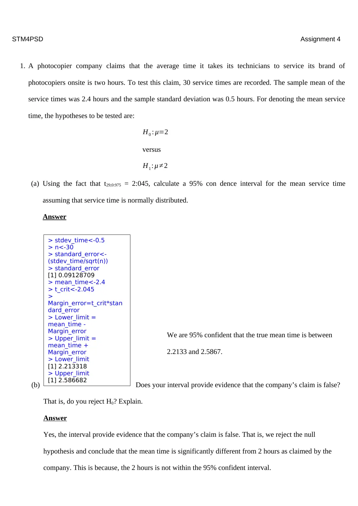
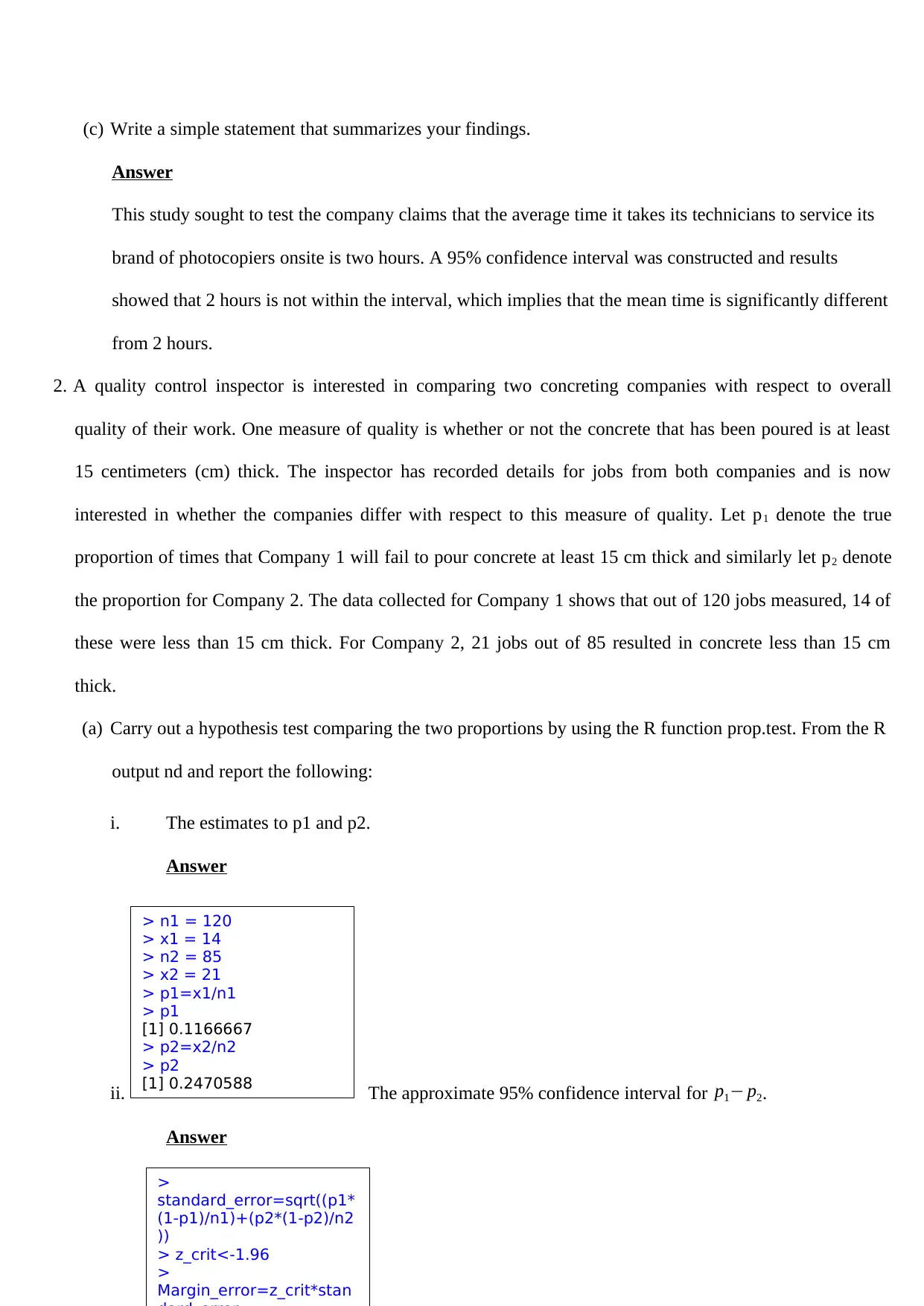
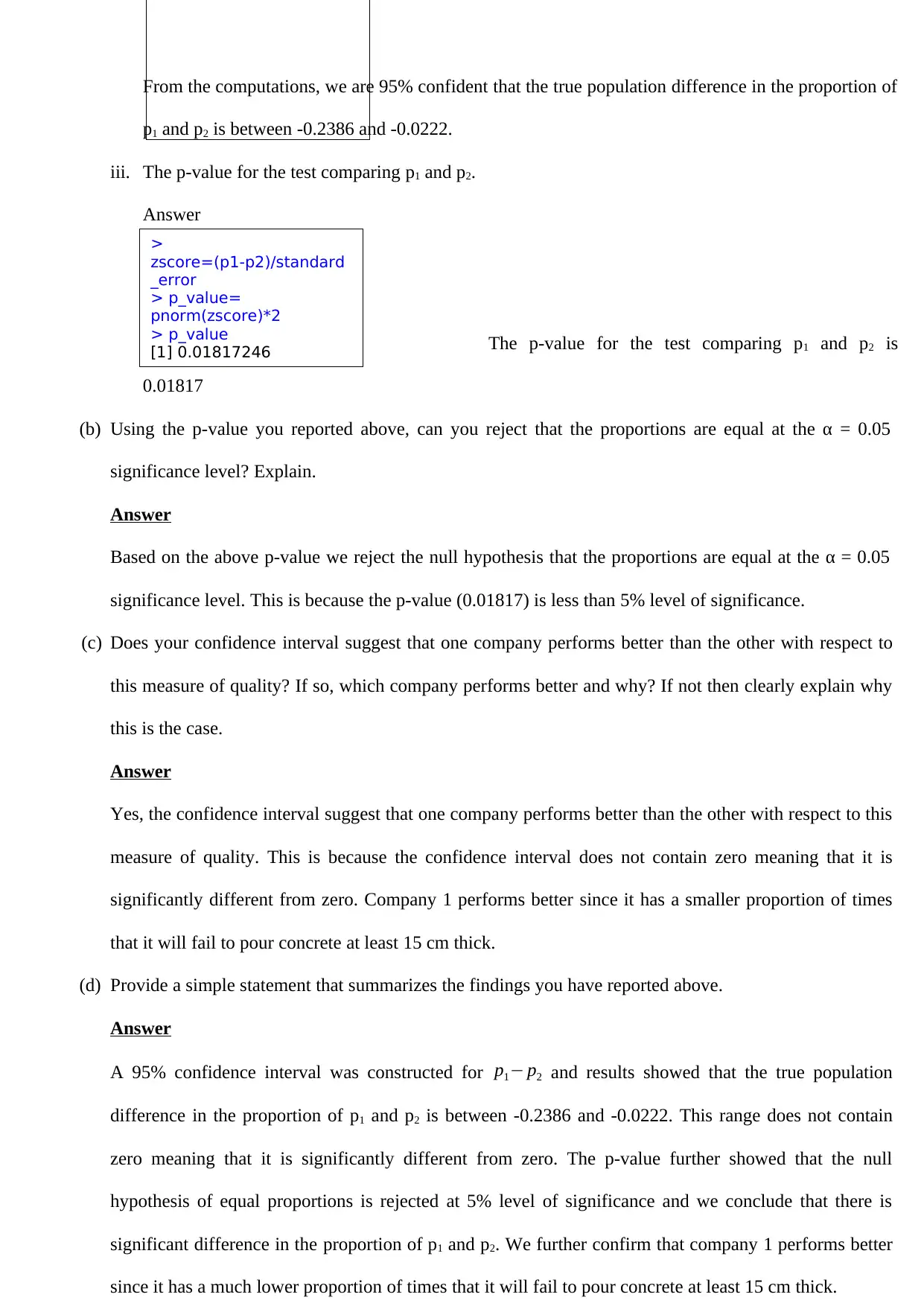
This assignment solution for STM4PSD Assignment 4 addresses several statistical problems. It begins by calculating a 95% confidence interval for the mean service time of a photocopier company's technicians, testing the company's claim. The solution then performs a hypothesis test to compare the proportions of jobs failing to meet quality standards between two concreting companies, utilizing the R function prop.test and interpreting the results. Finally, the assignment analyzes the 'Orange' dataset in R, creating scatter plots, boxplots, and performing linear regression to model the relationship between the age and circumference of orange trees, including residual analysis and interpretation of the regression model's fit. The document includes R code, outputs, and interpretations for all analyses, providing a comprehensive solution to the assignment's requirements.

Probability and Statistics
Student Name:
Instructor Name:
Course Number:
5th October 2019

STM4PSD Assignment 4
1. A photocopier company claims that the average time it takes its technicians to service its brand of
photocopiers onsite is two hours. To test this claim, 30 service times are recorded. The sample mean of the
service times was 2.4 hours and the sample standard deviation was 0.5 hours. For denoting the mean service
time, the hypotheses to be tested are:
H0 : μ=2
versus
H1 : μ ≠ 2
(a) Using the fact that t29;0:975 = 2:045, calculate a 95% con dence interval for the mean service time
assuming that service time is normally distributed.
Answer
We are 95% confident that the true mean time is between
2.2133 and 2.5867.
(b) Does your interval provide evidence that the company’s claim is false?
That is, do you reject H0? Explain.
Answer
Yes, the interval provide evidence that the company’s claim is false. That is, we reject the null
hypothesis and conclude that the mean time is significantly different from 2 hours as claimed by the
company. This is because, the 2 hours is not within the 95% confident interval.
> stdev_time<-0.5
> n<-30
> standard_error<-
(stdev_time/sqrt(n))
> standard_error
[1] 0.09128709
> mean_time<-2.4
> t_crit<-2.045
>
Margin_error=t_crit*stan
dard_error
> Lower_limit =
mean_time -
Margin_error
> Upper_limit =
mean_time +
Margin_error
> Lower_limit
[1] 2.213318
> Upper_limit
[1] 2.586682

(c) Write a simple statement that summarizes your findings.
Answer
This study sought to test the company claims that the average time it takes its technicians to service its
brand of photocopiers onsite is two hours. A 95% confidence interval was constructed and results
showed that 2 hours is not within the interval, which implies that the mean time is significantly different
from 2 hours.
2. A quality control inspector is interested in comparing two concreting companies with respect to overall
quality of their work. One measure of quality is whether or not the concrete that has been poured is at least
15 centimeters (cm) thick. The inspector has recorded details for jobs from both companies and is now
interested in whether the companies differ with respect to this measure of quality. Let p1 denote the true
proportion of times that Company 1 will fail to pour concrete at least 15 cm thick and similarly let p2 denote
the proportion for Company 2. The data collected for Company 1 shows that out of 120 jobs measured, 14 of
these were less than 15 cm thick. For Company 2, 21 jobs out of 85 resulted in concrete less than 15 cm
thick.
(a) Carry out a hypothesis test comparing the two proportions by using the R function prop.test. From the R
output nd and report the following:
i. The estimates to p1 and p2.
Answer
ii. The approximate 95% confidence interval for p1− p2.
Answer
> n1 = 120
> x1 = 14
> n2 = 85
> x2 = 21
> p1=x1/n1
> p1
[1] 0.1166667
> p2=x2/n2
> p2
[1] 0.2470588
>
standard_error=sqrt((p1*
(1-p1)/n1)+(p2*(1-p2)/n2
))
> z_crit<-1.96
>
Margin_error=z_crit*stan

From the computations, we are 95% confident that the true population difference in the proportion of
p1 and p2 is between -0.2386 and -0.0222.
iii. The p-value for the test comparing p1 and p2.
Answer
The p-value for the test comparing p1 and p2 is
0.01817
(b) Using the p-value you reported above, can you reject that the proportions are equal at the α = 0.05
significance level? Explain.
Answer
Based on the above p-value we reject the null hypothesis that the proportions are equal at the α = 0.05
significance level. This is because the p-value (0.01817) is less than 5% level of significance.
(c) Does your confidence interval suggest that one company performs better than the other with respect to
this measure of quality? If so, which company performs better and why? If not then clearly explain why
this is the case.
Answer
Yes, the confidence interval suggest that one company performs better than the other with respect to this
measure of quality. This is because the confidence interval does not contain zero meaning that it is
significantly different from zero. Company 1 performs better since it has a smaller proportion of times
that it will fail to pour concrete at least 15 cm thick.
(d) Provide a simple statement that summarizes the findings you have reported above.
Answer
A 95% confidence interval was constructed for p1− p2 and results showed that the true population
difference in the proportion of p1 and p2 is between -0.2386 and -0.0222. This range does not contain
zero meaning that it is significantly different from zero. The p-value further showed that the null
hypothesis of equal proportions is rejected at 5% level of significance and we conclude that there is
significant difference in the proportion of p1 and p2. We further confirm that company 1 performs better
since it has a much lower proportion of times that it will fail to pour concrete at least 15 cm thick.
>
zscore=(p1-p2)/standard
_error
> p_value=
pnorm(zscore)*2
> p_value
[1] 0.01817246

3. Suppose that the scientists are concerned with the growth of the orange trees in their area. Load the build-in
data called ‘Orange’ in R.
(a) Throughout we will assume that the data is stored in R as the data frame Orange.
Answer
(b) To visualize
(predictor) variable, create a scatter plot with a smooth line, utilizing the ‘scatter.smooth’ command.
Answer
The command used is as follows;
The plot is shown below;
The plot shows a positive linear relationship between age and circumference.
> data("Orange")
> head(Orange)
Tree age circumference
1 1 118 30
2 1 484 58
3 1 664 87
4 1 1004 115
5 1 1231 120
6 1 1372 142
> attach(Orange)
> scatter.smooth(age,
circumference, main =
"Circumference Vs. Age",
+ xlab = "Age",
ylab = "Circumference",
+ pch = 19)

(c) In order to check for outliers, produce two boxPlots of the variables ‘age’ and ‘circumference’, by
dividing the graph area in two columns, using the command ‘mfrow’.
Answer
The r code is given below;
The boxplots are shown below.
From the plots, it can be concluded that there are no outliers in either of the two variables (age or
circumference)
(d) Execute the following command to obtain least squares estimates and associated output in R.
lm.model <- lm(circumference ~ age, data = Orange)
summary(lm.model)
Provide a copy of your results displayed by summary(lm.model).
> par(mfrow=c(1,2))
> boxplot(age, main="Age", col="red")
> boxplot(circumference, main="Circumference", col="green")

Answer
(e) Create plots of the residual versus ts and the Q-Q plot of the standardised
residuals. Do you think the residuals versus fits plot or the Q-Q plot of
the residuals suggest that there are any linear regression model violations
that we need to be concerned with? Justify your answer with reference to
both of the plots.
NOTE: Regardless of your answer to (b), for the remainder of this
question please assume that there are no linear regression model
violations.
Answer
> lm.model <-
lm(circumference ~ age,
data = Orange)
> summary(lm.model)
Call:
lm(formula =
circumference ~ age,
data = Orange)
Residuals:
Min 1Q Median
3Q Max
-46.310 -14.946 -0.076
19.697 45.111
Coefficients:
Estimate Std.
Error t value Pr(>|t|)
(Intercept) 17.399650
8.622660 2.018
0.0518
age 0.106770
0.008277 12.900 1.93e-
14
(Intercept) .
age ***
---
Signif. codes:
0 ‘***’ 0.001 ‘**’ 0.01 ‘*’
0.05 ‘.’ 0.1 ‘ ’ 1
Residual standard error:
23.74 on 33 degrees of
freedom
Multiple R-squared:
0.8345, Adjusted R-
squared: 0.8295
F-statistic: 166.4 on 1
and 33 DF, p-value:
1.931e-14

The residuals versus fits plot or the Q-Q plot of the residuals suggest that there are no linear regression
model violations that we need to be concerned with. This is based on the fact that the plots shows that
the data is normality distributed and that there is constant variance for the residuals.
(f) Does the R output suggest that the regression model fits the data well? Explain.
Answer
The R output suggests that the regression model fits the data well. This is based on the fact that the p-
value for the F-statistic is less than 5% level of significance which leads to rejection of the null
hypothesis that the model is insignificant. Also, the value of R-Squared is 0.8345; this implies that
83.45% of the variation in the dependent variable (circumference) is explained by the independent
variable (age) in the model.